Reward the Stock as Well as the Flow: Notional Capitalized Value and Guarantee-Based Climate Incentives
Turning carbon stocks and low-emission paths into cheaper borrowing
Climate finance pays countries for marginal emission cuts measured against counterfactuals nobody can observe, and pays almost nothing for carbon stocks that were never released. This paper proposes a notional capitalized value: a balance opened by a country’s carbon stock, debited for every tonne emitted above an agreed allowance, and used not as cash but as guarantee capacity on its green borrowing. A guarantee saves the borrower the full credit spread but costs its provider only expected loss and the carry on a buffer, so on the development banks’ own sovereign loss record each dollar of expected loss buys about 80 dollars of interest saving. Net of the default option the borrower gives up, the figure is about 27; in a stress case without the banks’ preferred-creditor status it is 2.7, or 1.9 net. The stock should set the size of the balance and a separate price the debit per tonne. For a stylized forest country with Guyana’s carbon stock, a $5 billion balance saves $150 million a year and prices emissions at about $30 per tonne, at a donor cost of about 40 cents per tonne ($11 in the stress case). Capacity that declines as fast as technology costs fall is the cheapest way to make acting now beat waiting.
sovereign incentives, guarantees, carbon stocks, forest conservation, results-based climate finance, multilateral development banks
Working paper, version 0.2, October 2026. Stephen J. Stretton, writing in a personal capacity. The views expressed are the author’s own and do not represent those of any institution with which he is or has been affiliated. A short version for policy makers is Climate Fiscal Policy Brief No. 4.1.1
1 Executive summary
Policy brief (short version) → · Download this paper (pdf) · Slides (pdf)
Climate finance pays for the flow of emissions and almost nothing for the stock. Guyana’s forests hold about 19.5 billion tonnes of CO₂-equivalent. What Guyana sells is credits for emissions avoided against a reference level, about $50 million a year from Hess. Countries that never cleared have little to sell, generous baselines sell more, and the money arrives years after the political cost of reform. Donors will not vote cash on the scale stocks like Guyana’s would justify: Ecuador asked the world for $3.6 billion to leave an oil field unexploited and raised about $13.5 million.
The proposal is a notional capitalized value: a balance that the stock opens and emissions draw down. Each participating country gets an opening balance equal to its verified carbon stock times a low stock price. Each year the balance is debited at a higher, uniform debit price for every tonne the country emits above an agreed allowance, and credited for every tonne below. The balance is never paid out. It sets the country’s guarantee capacity: the maximum outstanding guarantee exposure that development banks, backed by a buffer fund, will provide on its eligible green borrowing.
A guarantee is worth much more to the borrower than it costs the guarantor. The country saves the spread between its own borrowing rate and the guaranteed rate; the guarantor bears only the expected loss. On the development banks’ record for sovereign lending (defaults of 0.77 percent a year, 95.1 percent recovered), a 3-point spread saving buys about $80 of interest saving per dollar of expected loss. Part of that saving is not a gain: a country that borrows under a guarantee backed by its own counter-indemnity gives up the option to default on that debt. Counting only the risk premium in the spread, about a third of it, the ratio is about 27. A new facility might not inherit the banks’ preferred-creditor status; in a stress case with 3 percent of guarantees called a year and 37 cents lost on the dollar, the ratios are 2.7 and 1.9.
The stock and the margin need different prices. Priced at $100 a tonne, Guyana’s stock would be a $1.95 trillion balance that no guarantor could back and that never binds, so an extra tonne would cost nothing. With the balance sized to a $5 billion borrowing need and a separate $50 debit per tonne, each tonne costs the country about $30 in lost interest savings: $32,500 per hectare cleared, against the $400–800 the Tropical Forest Forever Facility deducts. The country saves $150 million a year; donors hold a $25 million buffer and expect to lose about $2 million a year, 40 cents per tonne of incentive ($11 in the stress case). The $30 holds only while capacity binds and the scheme is open-ended, so surplus balance must flow to a beneficiary account.
The incentive scales with borrowing, not with the stock. Each $1 billion a year of incentive needs $33 billion of guarantee capacity, a buffer of $0.16 billion and about $13 million a year of expected losses on the banks’ record ($3.1 billion and $370 million in the stress case). The scheme is strong for large, lower-rated borrowers and weak for investment-grade or lightly indebted ones, for whom interest on the balance paid into a trust account is the better form.
Capacity that declines over time pays for acting now. Falling technology costs reward waiting. For a stylized $1 billion coal-to-renewables reform cutting 5 million tonnes a year, acting now needs an incentive of $20 a tonne ($32–37 allowing for uncertainty). Letting capacity decline as fast as technology costs fall halves the donor cost of that incentive, from $25 million to $13 million on the record. Paid in cash, it would cost $1 billion.
What to do. Development bank shareholders should create rules-based guarantee capacity outside country envelopes, allocated by notional capitalized value, with a uniform debit price and capacity sized to bind. Donors should fund the buffer, held in a trust, not the reward. Forest and coal countries should negotiate allowances, which change how much they get, rather than baselines, which change what they are paid for.
2 Introduction
Guyana’s forests store about 19.5 billion tonnes of CO₂-equivalent on some 18 million hectares (Government of Guyana 2022). At the $20 per tonne that Hess will pay, at least, on average for Guyana’s forest credits, that stock would be worth $390 billion. What Guyana sells instead is the gap between its emissions and a reference level. The Architecture for REDD+ Transactions (ART) issued it 33.47 million credits for 2016–2020, and Hess agreed to buy 2.5 million credits a year of vintages 2016–2030, 37.5 million in all, for at least $750 million (Department of Public Information, Guyana 2023), about $50 million a year. The stock enters only through a contested adjustment to the reference level that lets a high-forest, low-deforestation country credit against less than 0.05 percent of its stock a year (Integrity Council for the Voluntary Carbon Market 2026; Aster Global Environmental Solutions 2022). Leaving coal or oil in the ground earns nothing at all.
Two defects follow, and both are about the form of the reward rather than its size. First, paying for marginal tonnes against a counterfactual rewards whoever can claim the most generous baseline: an evaluation of voluntary forest-conservation projects found that most did not measurably reduce deforestation, and those that did reduced it far less than claimed (West et al. 2023). Second, the payment arrives after the result, often years after a government pays the political cost of reform, so it guards against reversal more than it starts anything (Angelsen 2017; Stretton 2026j, ch. 20). Paying more per tonne fixes neither defect, and donors will not vote cash on the scale that tropical forest stocks would justify. Ecuador’s Yasuní-ITT initiative asked for $3.6 billion over thirteen years to leave an oil field of about 920 million barrels unexploited, and had collected about $13.5 million when it was abandoned in 2013 (Hernández Rentería 2020).
This paper asks how the international system can give a government a large, early and credible incentive to protect carbon stocks and cut emissions without a cash transfer that donors will not vote for.
The answer is to credit each participating country with a notional capitalized value (NCV): an opening balance set by its carbon stock, debited for every tonne it emits above an agreed allowance and credited for every tonne below it. The balance is never paid out. It sets the country’s guarantee capacity, the maximum outstanding guarantee exposure that multilateral development banks (MDBs), backed by a buffer fund, will provide on the country’s eligible green borrowing. The country gains the spread it saves on guaranteed debt; donors bear the expected loss on the exposure and the carry cost of the buffer. Because each tonne emitted shrinks the balance, the incentive acts from the first year. Because capacity can be scheduled to decline, the reward is largest for acting early.
The paper makes four contributions.
- It derives what the incentive is worth and what it costs (Section 5.2). The ratio of interest saved to guarantor cost equals the spread saved divided by expected loss plus buffer carry: about 80 on the MDBs’ own sovereign loss record, 10 in a middle case and 2.7 in a stress case without preferred-creditor status. Because the country gives up its option to default on guaranteed debt, its economic gain is smaller than its budget saving: the risk premium in the spread plus the guarantor’s expected loss. With a premium of a third of the spread, the ratios are about 27, 4.3 and 1.9 (Proposition 1).
- It separates the two prices (Section 4.3, Section 5.3). A single notional price cannot both size the balance and price the margin. The stock should set the size of the balance and a uniform debit price the reward per tonne. The debit must be per tonne emitted and capacity must bind, or the marginal incentive is zero; when both hold, the incentive is a carbon price equal to the debit price times the spread over the discount rate (Proposition 2). The stock is what makes the debit enforceable: a sovereign will not pay a charge for emitting, but it can lose part of a balance it has not drawn.
- It prices acting now (Section 5.4). Acting now beats waiting if and only if the initial incentive per tonne covers the interest and technology-cost return to waiting, and the cheapest schedule that achieves this lets capacity decline at the rate technology costs fall (Proposition 3).
- It calibrates the scheme (Section 6) for a forest country with Guyana’s verified stock, for a coal country with Indonesia’s reserves, and for the scale needed to make an incentive large. It corrects the arithmetic of the original proposal, which understates its own incentive tenfold.
The closest work is of three kinds. ART’s high-forest, low-deforestation (HFLD) crediting and the earlier proposal of “preventive credits” for such countries (Fonseca et al. 2007) reward stocks by raising the baseline against which avoided emissions are counted, which is why they are contested on additionality (Integrity Council for the Voluntary Carbon Market 2026). The Tropical Forest Forever Facility (TFFF) pays forest countries per hectare of standing forest out of the spread on a leveraged bond portfolio (Government of Brazil 2025). And the theory of conservation contracts shows that paying an owner to conserve can fail, because the owner gains from threatening to exploit (Harstad 2016). This paper differs from all three in delivering the reward through guarantees, where the gap between the borrower’s value and the provider’s cost creates the leverage; in fixing the stock reward at entry and pricing every tonne released at a uniform rate, which removes both the baseline game and the gain from threats; and in deriving when the reward changes what a government does and when it does it.
3 Literature and precedents
Results-based forest finance pays for flows against reference levels. The Paris Agreement encourages results-based payments for reducing emissions from deforestation and forest degradation (REDD+) (UNFCCC 2015, Article 5.2). A review of Norway’s partly performance-based agreements with Brazil, Guyana, Indonesia and Tanzania identifies reference levels, performance criteria, risk sharing and the credibility of funding as the main design problems of results-based aid (Angelsen 2017). Jurisdictional standards such as ART-TREES moved crediting from projects to national or subnational territories, which removes within-country leakage and makes the counterfactual a national rather than a project baseline. Guyana is the leading case: 33.47 million credits for 2016–2020, of which Hess buys 2.5 million a year at $15 per tonne for the first vintages, under a contract worth at least $750 million (Department of Public Information, Guyana 2023). The price is modest, the stream is long, and the payment is for avoided flow.
Baselines are the weak point, and the stock is rewarded by bending them. An evaluation of 26 voluntary forest-conservation projects using synthetic controls found that most did not significantly reduce deforestation and that claimed reductions far exceeded measured ones (West et al. 2023). Jurisdictional baselines are harder to game but face the same logic: a country whose deforestation was always low has little to sell, and a country that raised deforestation before the baseline period is rewarded for lowering it again (Stretton 2026j, ch. 20). To include low-deforestation countries, Fonseca et al. (2007) proposed “preventive credits” against a reference rate indexed to the global deforestation rate. ART’s HFLD approach does something similar: it adds to measured reductions a credit on less than 0.05 percent of the standing stock a year, as if that much were at risk (Integrity Council for the Voluntary Carbon Market 2026). Guyana’s 2016–2020 credits used this approach, with a crediting level of 22.6 million tonnes a year (Aster Global Environmental Solutions 2022). The integrity council for the voluntary market has made approval of these credits conditional on remedial action, because the adjustment is hard to show to be additional (Integrity Council for the Voluntary Carbon Market 2026). This is a stock reward presented as an avoided-emissions credit, and it inherits the credibility problems of both.
Stock-based payments exist but are small. The TFFF, launched by Brazil on 6 November 2025 with the World Bank as trustee and interim host (Barber et al. 2025), aims to raise $25 billion of sponsor capital and up to $100 billion of senior debt from market investors. Sponsor capital is repaid over 30 years after a 10-year grace period, at a cost assumed not to exceed US Treasury yields; the fund invests in a diversified portfolio of rated bonds and, after servicing its debt and paying sponsors, pays forest countries about $4 per hectare of eligible forest a year, with at least 20 percent going to Indigenous peoples and local communities, for countries whose deforestation stays at or below 0.5 percent a year (Government of Brazil 2025). Each hectare deforested cuts the payment by the equivalent of 100 hectares where deforestation is at or below 0.3 percent a year, and of 200 hectares between 0.3 and 0.5 percent; each hectare degraded by fire cuts it by 35 (Government of Brazil 2025). Sponsors had pledged $6.7 billion by late November 2025, and 74 developing countries are eligible (Barber et al. 2025). The TFFF is the first large instrument that pays for the stock directly. It is also, in effect, interest on a notional value, one of the four NCV formulations reconciled in Section 4.2, with the leverage on the investment side rather than the guarantee side.
Paying owners to conserve can fail, and how it fails matters for design. Payments for environmental services work when the payment exceeds the landholder’s opportunity cost and is conditional on the service (Engel et al. 2008). But Harstad (2016) shows that when a buyer pays an owner to conserve, the owner’s ability to threaten exploitation undermines the market: conservation is less likely the more valuable it is, and with a patient owner who sets the price the forest is eventually lost. Any stock payment that rises with the threat to the stock invites this hold-up. On the fossil side, Harstad (2012) shows that buying and conserving deposits in non-participating countries addresses leakage through the fuel market; Collier and Venables (2014) argue for closing coal in sequence, starting with rich countries; and Asheim et al. (2019) argue that a treaty limiting fossil fuel supply would strengthen the Paris Agreement. Cash for stocks has been tried: Ecuador’s Yasuní-ITT initiative raised under 0.4 percent of what it asked (Hernández Rentería 2020).
Guarantees and the cost of capital. Developing countries face substantially higher costs of capital for renewable power than industrialized ones (Steffen 2020), and that gap alone can lock them into higher-carbon paths (Ameli et al. 2021). A loan guarantee is a put option on the borrower’s assets (Merton 1977); its value to the borrower is the market’s price of that option, while its cost to the guarantor is the guarantor’s own expected loss. The two diverge for two reasons. Sovereign spreads include a risk premium, about a third of the spread on average, on top of compensation for expected default losses (Longstaff et al. 2011). And MDBs are senior creditors in practice (Schlegl et al. 2019): their sovereign and sovereign-guaranteed loans defaulted at 0.77 percent a year over 1984–2024, with 95.1 percent recovered (European Investment Bank 2025), an expected loss of about 0.04 percent a year, while the same sovereigns pay market spreads of several hundred basis points. Gabon’s 2023 debt-for-nature swap shows the gap: a $500 million bond carrying US political risk insurance paid a 6.097 percent coupon and was rated Aa2, fourteen notches above the sovereign’s Caa1 (African Sovereign Debt Justice Network 2023), when Gabon’s 2031 bonds yielded about 10 percent (Smith 2023). Seniority also has a cost to others: Chamon et al. (2022) show that debt-for-climate swaps are generally less efficient than conditional grants because part of the benefit leaks to creditors outside the deal, unless the climate commitment is made de facto senior.
Clubs and timing. A climate club works by offering members a benefit that non-members lose (Nordhaus 2015). Cheaper borrowing is such a benefit, and unlike trade penalties it costs the club little to supply. On timing, the theory of irreversible investment under uncertainty shows that the option to wait raises the hurdle for acting now above the simple net-present-value rule (Dixit and Pindyck 1994). Falling technology costs make waiting more attractive still, so an incentive that is constant over time is weakest exactly when action is most valuable.
The gap. No existing instrument rewards the stock without bending a baseline, prices each tonne released at a uniform rate, arrives before the policy cost is paid and costs donors much less than it is worth. Results-based payments price the margin but pay late and against baselines. HFLD crediting and the TFFF pay for the stock, the first through a contested baseline and the second at a few dollars per hectare. Guarantees are cheap to supply but are allocated by project and lending envelope, not by climate performance. This paper joins the three.
4 The notional capitalized value
4.1 Definition: a balance that the stock opens and emissions draw down
A country’s notional capitalized value is a climate balance held for it by an international arrangement. It opens at the value of the country’s carbon stock and moves each year with its emissions:
\[B_0 = p_s S_0, \qquad B_{t+1} = B_t + p_e\,(A_t - E_t), \qquad B_t \ge 0. \tag{1}\]
Here \(S_0\) is the verified carbon stock at entry in tonnes of CO₂ (forest carbon, and optionally fossil reserves legally retired), \(p_s\) is the stock price in dollars of opening balance per tonne of stock, \(E_t\) is the country’s emissions in year \(t\) from all sources including land use, \(A_t\) is its allowance, an agreed benchmark path, and \(p_e\) is the debit price in dollars per tonne. Emitting above the allowance debits the balance; emitting below it credits the balance. Deforestation enters through \(E_t\) as land-use emissions, so the forest stock is not revalued each year; every tonne emitted, from a chimney or a cleared hectare, costs the same \(p_e\).
The balance is notional. Nobody claims that Guyana’s forests could be sold for \(p_s S_0\); the number is an agreed basis for an entitlement (Stretton 2026j, ch. 21). The idea has a mirror image in liability law: an emission inflicts damage on identifiable people in the future, so the prudent response is to provision for it, which makes it a capital requirement rather than an expense (Stretton 2026i, ch. 7). The NCV applies the same accounting to the country that holds a stock: an unreleased stock is notional capital, and each tonne released is a withdrawal from it.
The balance sets guarantee capacity:
\[G_t = \lambda_t B_t, \qquad X_t = \min(G_t, D_t), \tag{2}\]
where \(\lambda_t\) is the capacity ratio (dollars of guarantee capacity per dollar of balance, possibly declining over time), \(D_t\) is the country’s outstanding eligible green borrowing, and \(X_t\) is the exposure actually guaranteed.
4.2 Four formulations, reconciled
Earlier drafts contain four versions of the idea. Table 1 sets them side by side.
| Version and source | What the country gets | Stock base | Annual adjustment | Role here |
|---|---|---|---|---|
| Interest on a notional value (Climate Investment Trust drafts; Time and Chance ch. 20) | Interest on, say, a $1tn Amazon valuation, paid into a trust account | Forest; coal in one draft | Not specified | Variant for countries that do not borrow (Section 7) |
| Notional Capitalized Carbon Value (Time and Chance ch. 21) | Guarantee capacity released over ten years | Forest, unburned fossil fuel | Minus price × net emissions | Main form, with arithmetic corrected (Section 6.2) |
| Climate balance on stocks and long-run emissions (research page) | Guarantee support, used up by business-as-usual emissions | Stocks and long-run path | Debited by business-as-usual emissions | Main form; the debit made per tonne |
| Climate allowance of guarantee capacity (DPhil proposal) | Rules-based guarantee capacity adjusted with performance | Not specified | Rises with early action, falls when targets are missed | The release schedule of Proposition 3 |
The four versions agree on the core and differ on three choices, which this paper settles.
Reward form: guarantee capacity, not interest. Interest paid into an account is cash, deferred; it costs donors a dollar per dollar of incentive. Guarantee capacity costs a fraction of its value (Proposition 1). It also arrives when a government needs it, as cheaper borrowing for the investments the policy requires, rather than years after the result. Interest into a trust account remains the right form for countries that do not borrow in volume, such as small island states without bond market access or a country whose oil revenue makes borrowing unnecessary.
Capacity is a cap on outstanding exposure, not a flow of new guarantees. The original arithmetic did not say which, and the difference is a factor of ten (Section 6.2). A cap on outstanding exposure is the natural reading of a balance, matches how MDBs manage guarantee limits, and gives the debit a clean meaning: every dollar debited is a dollar less of exposure the country can have guaranteed from then on.
The debit is per tonne emitted, against an allowance, at its own price. “Used up by business-as-usual emissions” could mean a fixed draw-down set by a forecast. That would have no effect on behavior (Proposition 2). The debit must move with actual emissions. Setting the debit price separately from the stock price is the main change from all four drafts.
4.3 Why the stock and the debit need different prices
A single price cannot both size the balance and price the margin. Suppose \(p_s = p_e = p\). For the debit to bite, capacity must bind: the country must want more guarantee capacity than it has, so \(\lambda B_t < D_t\). With Guyana’s stock of 19.5 billion tonnes and eligible borrowing of, say, $5 billion, a binding balance requires \(p < \$0.26\) per tonne, and the marginal tonne is then worth about $0.15 to the country (Section 6.3). At the $100 per tonne of the original proposal, the balance is $1.95 trillion, capacity never binds, and the marginal tonne is worth nothing.
The two prices do different jobs. The stock price decides how much capacity each country starts with, which is a question of distribution and of what the country stands to lose. The debit price decides what each tonne costs, which is the question of incentives. Separating them lets the stock reward large forest countries without paying them for tonnes they were never going to emit, and lets the debit price be set high enough to change behavior without creating a balance no guarantor could stand behind.
The stock still matters at the margin, for a reason the separation makes clear. An international feebate between countries founders on negative transfers, because no sovereign will write a check for exceeding its benchmark; a deduction from a balance held in trust is enforceable where a payment is not (Stretton 2026i, ch. 5). The opening balance is what the debit is deducted from. Without a stock there is nothing to debit; with one, a country that emits loses something it already counts as its own.
Fixing the opening balance at entry also answers the hold-up problem of Harstad (2016). In a market for conservation the owner is paid more the more credibly it threatens to exploit, so threats pay. Under the NCV the opening balance depends on the verified stock at entry, not on the threat to it, and the reward for not emitting is the uniform debit price, the same for every country and every tonne. A country cannot raise either by threatening to clear.
5 Model
5.1 Setup
A country holds balance \(B_t\) under equation 1 and capacity \(G_t\) under equation 2. Guaranteed borrowing pays the guarantor’s rate rather than the market rate, saving \(\Delta s\) per dollar of guaranteed exposure per year. The guarantor’s annual expected loss per dollar of exposure is \(\pi L\), the probability of a call times the loss per call. Behind the guarantees sits a buffer fund holding \(k\) dollars of capital per dollar of exposure; holding it costs \(\varphi\) a year per dollar, the donors’ opportunity cost of funds net of what the buffer earns. The guarantor may charge a fee \(f\) per dollar of exposure. Time is discrete in Proposition 1 and continuous in Propositions 2 and 3, with discount rate \(r\) and discount factor \(\delta = 1/(1+r)\).
The incentive value to the country is the present value of spread saved, net of fees:
\[V = \sum_t \delta^t (\Delta s - f) X_t. \tag{3}\]
The cost to the guarantor and donors is expected loss plus buffer carry, net of fees:
\[C = \sum_t \delta^t (\pi L + k\varphi - f) X_t. \tag{4}\]
5.2 Proposition 1: a guarantee is worth several times what it costs
Proposition 1 (incentive-to-cost ratio). Let \(\Delta s\), \(\pi L\), \(k\), \(\varphi\) and \(f\) be constant over the life of the exposure.
(a) For any path of guaranteed exposure,
\[\frac{V}{C} = R \equiv \frac{\Delta s - f}{\pi L + k\varphi - f}. \tag{5}\]
A guarantee delivers more incentive per dollar of donor cost than a grant (\(R > 1\)) if and only if \(\Delta s > \pi L + k\varphi\). A fee \(f = \pi L + k\varphi\) makes the scheme self-financing while the country keeps \(\Delta s - \pi L - k\varphi\) a year per dollar of exposure.
(b) Suppose the market spread is the market’s expected default loss plus a risk premium \(\rho\), and the country, which counter-indemnifies the guarantor, gives up its option to default on the guaranteed debt except to the extent the guarantor itself loses. Then the country’s economic gain per dollar of exposure a year is \(\rho + \pi L - f\), and
\[\frac{V_e}{C} = R_e \equiv \frac{\rho + \pi L - f}{\pi L + k\varphi - f} \;\le\; R . \tag{6}\]
The proofs are in Appendix A. Part (a) is the budget ratio: what a finance ministry sees each year as lower interest bills. It does not depend on the size or timing of the exposure, so it is the right statistic for comparing a guarantee with a grant, for which \(R = 1\). Part (b) is the economic ratio. Under market debt a country in distress imposes a haircut on its creditors; under a guarantee backed by its counter-indemnity it owes the guarantor instead, and on the MDB record repays almost all of it. The part of the spread that paid creditors for bearing default is therefore not a gain to the country, only the risk premium and whatever loss the guarantor still bears. Part (b) is a lower bound, because it ignores the output and access costs of a market default that the country also avoids (Cruces and Trebesch 2013).
Why should the spread saved exceed the guarantor’s cost? Because the market prices the sovereign’s risk to all creditors, plus a premium, while the guarantor bears only the sovereign’s risk to it. MDBs are senior creditors in practice (Schlegl et al. 2019) and, for guarantees with a sovereign counter-indemnity, hold a claim the government has strong reasons to honor. Their record bears this out: sovereign and sovereign-guaranteed loans defaulted at 0.77 percent a year over four decades and recovered 95.1 percent (European Investment Bank 2025). The resource being spent is the gap between the risk the guarantor actually bears and the risk the market charges for (Stretton 2026j, ch. 21). It needs no appropriation, but it is not free: losses will occur, and a buffer must stand behind the exposure.
This paper takes that record as its base case, shared with the companion papers on the Climate Investment Trust and sustainability-linked lending (Stretton 2026h, 2026b): a 0.77 percent annual probability that a guarantee is called and a 4.9 percent loss when it is (one minus the 95.1 percent recovery), for an expected loss of 0.038 percent a year (European Investment Bank 2025). A buffer of 0.5 percent of exposure then keeps the annual chance of exhausting it at 1 percent across 20 guaranteed programs with asset correlation 0.2; it covers two calls in the same year. The buffer is invested in safe assets and earns the rate used to discount, so its carry cost is zero (\(\varphi = 0\)). With \(\Delta s\) = 3 percent, \(R\) = 3/0.038, about 80. With a risk premium of a third of the spread (Longstaff et al. 2011), \(\rho\) = 1 percent and \(R_e\) = 1.038/0.038, about 27.
The record is not a promise that a new facility can keep. It reflects the MDBs’ preferred-creditor status: governments in distress keep paying the development banks while they restructure other debt. A climate guarantee facility might not inherit that status, especially if its guarantees cover market debt rather than MDB loans. So the paper reports two less favorable cases with the same correlation, number of programs and exhaustion target. In a middle case, a call is about four times as likely (3 percent a year) and loses 10 percent; \(R\) = 10 (\(R_e\) = 4.3), and the buffer is 2.5 percent of exposure. In a stress case, calls occur at 3 percent a year and lose 37 percent, the average investor haircut in sovereign restructurings over 1970–2010 (Cruces and Trebesch 2013), an expected loss of 1.11 percent a year, nearly 30 times the MDB record; the buffer is 9.3 percent of exposure and \(R\) = 2.7 (\(R_e\) = 1.9) (Stretton 2026h). Charging the buffer a 2 percent carry cost lowers \(R\) to 63 in the base case and 2.3 in the stress case. Because a buffer invested at the discount rate costs nothing net, a facility can price its guarantees on the record and still hold the stress-case buffer until it has a record of its own. That holds only at zero carry: if the buffer costs 2 percent a year to hold, pricing on the record while holding the stress-case buffer gives a ratio of about 13, not 80. The ratios also assume the exposure is held indefinitely, so the buffer is consumed only by losses (Stretton 2026h).
5.3 Proposition 2: the debit must be per tonne, and capacity must bind
The marginal incentive is what changes behavior. Let capacity bind on an interval of time, meaning \(0 < \lambda_t B_t < D_t\), so every extra dollar of capacity is used and every dollar lost reduces guaranteed exposure. Let the capacity ratio decline at rate \(\theta \ge 0\), \(\lambda_t = \lambda_0 e^{-\theta t}\).
Proposition 2 (incentive compatibility and the carbon-price equivalent).
(a) If capacity binds from time \(s\) onward, a tonne emitted at \(s\) costs the country, in present value at \(s\),
\[\tau(s) = \frac{\lambda_0\, p_e\, (\Delta s - f)}{r + \theta}\, e^{-\theta s}. \tag{7}\]
This is the carbon-price equivalent of the scheme: the uniform carbon price that gives the same reward for cutting a tonne.
(b) If the debit is fixed in advance from a forecast of business-as-usual emissions rather than charged per tonne emitted, the marginal incentive is zero.
(c) The allowance path \(A_t\) does not enter \(\tau(s)\). It changes the level of the balance, and so who gains, but not the reward per tonne.
(d) If capacity does not bind, because \(\lambda_t B_t \ge D_t\) (the country has more capacity than borrowing) or \(B_t = 0\) (the balance is exhausted), the marginal incentive in those years is zero.
The proof is in Appendix A. Part (a) gives the conversion rate from notional to effective price: with no decline in capacity and \(\lambda_0 = 1\), each dollar of debit price is worth \(\Delta s/r\) dollars of carbon price, 60 cents at a 3 percent spread and a 5 percent discount rate. A government that cuts emissions until the marginal cost of a cut equals its marginal reward makes the same cut under the NCV as under a uniform carbon tax of \(\tau\), so \(\tau\) is the carbon-price equivalent in the sense of the series’ Total Effective Carbon Price (Stretton 2026e), and the NCV can be compared directly with a tax, a feebate or policy crediting. The donors’ cost per dollar of carbon-price equivalent is \((\pi L + k\varphi)/\Delta s\): about 1.3 cents in the base case and 37 cents in the stress case.
Part (a) also states its conditions, and both matter in practice. The formula assumes capacity binds from \(s\) for ever. If the scheme ends at a fixed date, the price falls as the date approaches: at a $50 debit price, a tonne emitted in 2027 under a scheme that ends in 2050 costs $20 rather than $30, and one emitted in 2040 costs $12. The scheme must therefore be open-ended, or its balance must end in something the country still values, such as a beneficiary account.
Part (b) is the reason the debit must be per tonne emitted. A schedule that draws the balance down by business-as-usual emissions whatever the country does is a declining transfer, and a transfer changes nothing at the margin. “Used up by business-as-usual emissions” must mean that business-as-usual emissions would use it up, not that they are assumed to.
Part (c) turns the hardest dispute in results-based finance, the baseline, into a question of distribution. A generous allowance gives a country more balance, but each tonne still costs \(p_e\). Negotiators can trade allowance against participation without weakening the incentive. That is not true of crediting against a baseline, where an inflated baseline pays for tonnes that were never at risk, nor of HFLD crediting, where the stock reward is delivered by inflating the baseline.
Part (d) gives two design rules. Capacity must be sized to the country’s borrowing, so that it binds; surplus balance above \(D_t/\lambda_t\) should flow somewhere it still has value, such as a beneficiary account in the Climate Investment Trust (Stretton 2026g). And the allowance must keep the balance positive along a path the country can reach, because a country that expects to exhaust its balance has no incentive in the years after exhaustion and a weaker one before.
5.4 Proposition 3: paying for acting now
A government chooses when to adopt a policy, such as a coal-retirement program or a forest-enforcement regime. Adopting at time \(T\) costs \(K_0 e^{-gT}\) up front, a cost that falls at rate \(g\) as technology improves, and cuts emissions by \(\Delta E\) tonnes a year from then on. The country values each tonne abated at \(b\) (domestic co-benefits, such as cleaner air) and bears an ongoing cost of \(\omega\) per tonne (for example, agricultural rent forgone on protected forest). Under the NCV each tonne abated at time \(s\) is worth \(m(s)\) to the country, the carbon-price equivalent of equation 7, written here in the general declining form \(m(s) = m_\infty + (m_0 - m_\infty)e^{-\theta s}\) with a floor \(m_\infty \ge 0\). The net present value of adopting at \(T\) is
\[W(T) = \int_T^\infty \Delta E\,[m(s) + b - \omega]\,e^{-rs}\,ds \;-\; K_0 e^{-(r+g)T}. \tag{8}\]
Proposition 3 (early action). Suppose the persistence condition \(m_\infty + b \ge \omega\) holds and the incentive declines no faster than technology costs, \(\theta \le g\). Then acting now (\(T = 0\)) is optimal if and only if
\[\Delta E\,(m_0 + b - \omega) \;\ge\; (r + g)\,K_0. \tag{9}\]
The minimum initial incentive is \(m_0^* = (r+g)K_0/\Delta E + \omega - b\). Holding \(m_0 = m_0^*\), the donor cost of the incentive falls as \(\theta\) rises, so among schedules satisfying the conditions the cheapest declines at \(\theta = g\) toward the floor \(m_\infty = \max(\omega - b, 0)\).
The proof is in Appendix A. The condition has a plain reading. Waiting a year saves interest on the up-front cost (\(rK_0\)) and lets the cost fall (\(gK_0\)); acting a year sooner earns a year of net benefit from the abated tonnes. Falling technology costs raise the hurdle: the faster solar or storage costs fall, the more a government gains by waiting, and the bigger the early incentive must be. Without an incentive, a government whose co-benefits do not exceed its ongoing costs (\(b \le \omega\)) never acts. One whose co-benefits do exceed them acts, but late: only once the cost has fallen to the point where \(\Delta E\,(b - \omega)e^{gT} = (r+g)K_0\), that is at \(T^* = \tfrac1g \ln\left[(r+g)K_0/(\Delta E(b - \omega))\right]\). The incentive’s job is to bring \(T^*\) forward to zero.
The persistence floor separates two cases. For an energy transition, the ongoing cost of keeping clean capacity is close to zero once it is cheaper than coal, so \(\omega \approx 0\) and the incentive can phase out: the reward is needed to start, not to continue. For forests, the opportunity cost of standing forest persists as long as there is demand for land, so \(\omega > 0\) and the floor stays: a forest needs a permanent price, an energy transition a temporary early one. A single scheme can serve both because the floor and the decay are parameters, not constants.
Uncertainty raises the hurdle further. If the up-front cost follows a driftless random walk, the standard result is that the trigger rises by a factor \(\beta/(\beta - 1) > 1\), where \(\beta\) depends on volatility and the discount rate (Dixit and Pindyck 1994, ch. 5). With a 5 percent discount rate and volatility of 15–20 percent a year, the factor is 1.6–1.9 (author’s calculation, Appendix B), so the initial incentive in equation 9 must be 60–90 percent larger. The decaying schedule is the instrument for this: a government that knows capacity per tonne falls each year it delays faces a cost of waiting that the market alone does not impose. This is the early-action premium of the series, built into the release schedule.
5.5 Three quantities, kept apart
The framework keeps apart three quantities that discussions of climate finance often merge (Stretton 2026f). Mitigation effectiveness is \(\Delta E\): the emissions cut that a policy produces. The sovereign incentive required is \(m_0^*\) in equation 9: the reward per tonne that makes acting now worth more than waiting. The resource cost to MDBs and donors is \(m_0^* (\pi L + k\varphi)/\Delta s\) per tonne: what it costs to create that incentive through guarantees. A grant makes the third quantity equal to the second; a guarantee divides it by \(R\).
6 Calibration
6.1 Parameters
Table 2 lists the values used. Anchored values come from published sources; stylized values are assumptions, labeled as such, and the code in Appendix B reproduces every number.
| Parameter | Symbol | Value | Basis |
|---|---|---|---|
| Spread saved on guaranteed debt | \(\Delta s\) | 3.0 pp (1.5–4.5) | Stylized; Gabon 2023: insured bond at 6.097% against about 10% on its 2031 bonds, a saving of about 3.9 pp before the insurance premium (African Sovereign Debt Justice Network 2023; Smith 2023) |
| Risk premium in the spread | \(\rho\) | 1.0 pp (a third of \(\Delta s\)) | Average share of sovereign spreads (Longstaff et al. 2011) |
| Guarantor’s expected loss | \(\pi L\) | 0.038% a year (0.30%; 1.11%) | Base case: MDB record, 0.77% annual calls × 4.9% loss (European Investment Bank 2025); in brackets, middle case (3% × 10%) and stress case (3% × 37%) (Stretton 2026h; Cruces and Trebesch 2013) |
| Buffer per dollar of exposure | \(k\) | 0.5% (2.5%; 9.3%) | 1% annual chance of exhaustion, 20 programs, correlation 0.2 (Stretton 2026h) |
| Net carry cost of buffer | \(\varphi\) | 0 (2% in sensitivity) | Buffer invested at the discount rate |
| Discount rate | \(r\) | 5% | Stylized |
| Fee | \(f\) | 0 | Baseline; cost-covering fee considered |
| Debit price | \(p_e\) | $50 per tCO₂ | Stylized |
| Forest carbon stock | \(S_0\) | 19.5 GtCO₂e on 18 Mha | Guyana (Government of Guyana 2022) |
| Eligible green borrowing (forest country) | \(D\) | $5 billion | Stylized |
The spread saved is the most important input and the most country-specific. Three percentage points is a little below the saving Gabon achieved with insurance on a single bond, and is the figure used in the original proposal (Stretton 2026j, ch. 21). It applies to a country rated well below investment grade. For an investment-grade sovereign the saving is smaller; this paper assumes 1 percentage point, and the case for guarantees is weaker (Section 6.5).
6.2 Correcting the original arithmetic
The original proposal values a forest stock of 100 MtCO₂ at $100 per tonne, a balance of $10 billion, debited by $100 million for each million tonnes emitted. It releases the balance over ten years, “roughly $1 billion of NCCV capacity per year”, and, at a saving of 3 percent per dollar guaranteed, finds “$30 million in annual interest-cost reductions” and $300 million over ten years (Stretton 2026j, ch. 21). The text does not say whether the $1 billion is a cap on outstanding exposure or a flow of new guarantees each year. Table 3 shows that the answer changes the incentive tenfold.
| Reading | Outstanding guaranteed exposure | Annual saving | Total saving | Present value at 5% | Price of a tonne emitted |
|---|---|---|---|---|---|
| A. $1bn cap on outstanding exposure for 10 years | $1bn | $30m | $0.3bn | $0.23bn | $0 (capacity slack) |
| B. $1bn of new 10-year guarantees each year for 10 years | Rises to $10bn | $30m rising to $300m | $3.0bn over the loans’ lives | $1.88bn | Depends on which year’s issue is cut |
| C. Whole $10bn balance as a cap from year 1 | $10bn | $300m | $3.0bn over 10 years | $2.32bn | About $21/t with 9 years left |
The $30 million and $300 million figures are correct only under reading A, and reading A is the worst design. With $1 billion of capacity against a $10 billion balance, capacity does not bind until the country has emitted 90 MtCO₂, so for decades an extra tonne costs nothing (Proposition 2(d)). Under reading C, the natural reading of a balance, the incentive is $300 million a year and each tonne emitted costs about $21 in lost spread savings. The correction does not change the donor cost per dollar of incentive, which Proposition 1 sets; it changes how much incentive a given balance delivers, by a factor of ten.
6.3 A forest country
Take a stylized forest country with Guyana’s verified stock: 19.5 billion tonnes of CO₂-equivalent on about 18 million hectares, an average of about 1,080 tonnes per hectare (Government of Guyana 2022). Give it $5 billion of eligible green borrowing (stylized), a stock price that opens the balance at that level (\(p_s\) = $0.26 per tonne), a debit price of $50 per tonne, and emissions of 15 MtCO₂ a year from all sources against an allowance that falls from 12 Mt in 2027 to zero in 2050 (stylized).
Incentive and cost. With capacity fully used, the country saves $150 million a year, $1.87 billion in present value over 20 years. On the MDB record, donors hold a buffer of $25 million and bear an expected annual cost of about $2 million; in the stress case the buffer is $0.47 billion and the cost $56 million. While capacity binds in an open-ended scheme, each tonne emitted costs the country $30 in lost spread savings ($50 × 3% ÷ 5%), and each hectare cleared about $32,500. Donors’ cost per tonne of that carbon-price equivalent is about 40 cents in the base case, $3 in the middle case and $11 in the stress case, against the $15–20 per tonne Hess pays in cash for credits against a reference level.
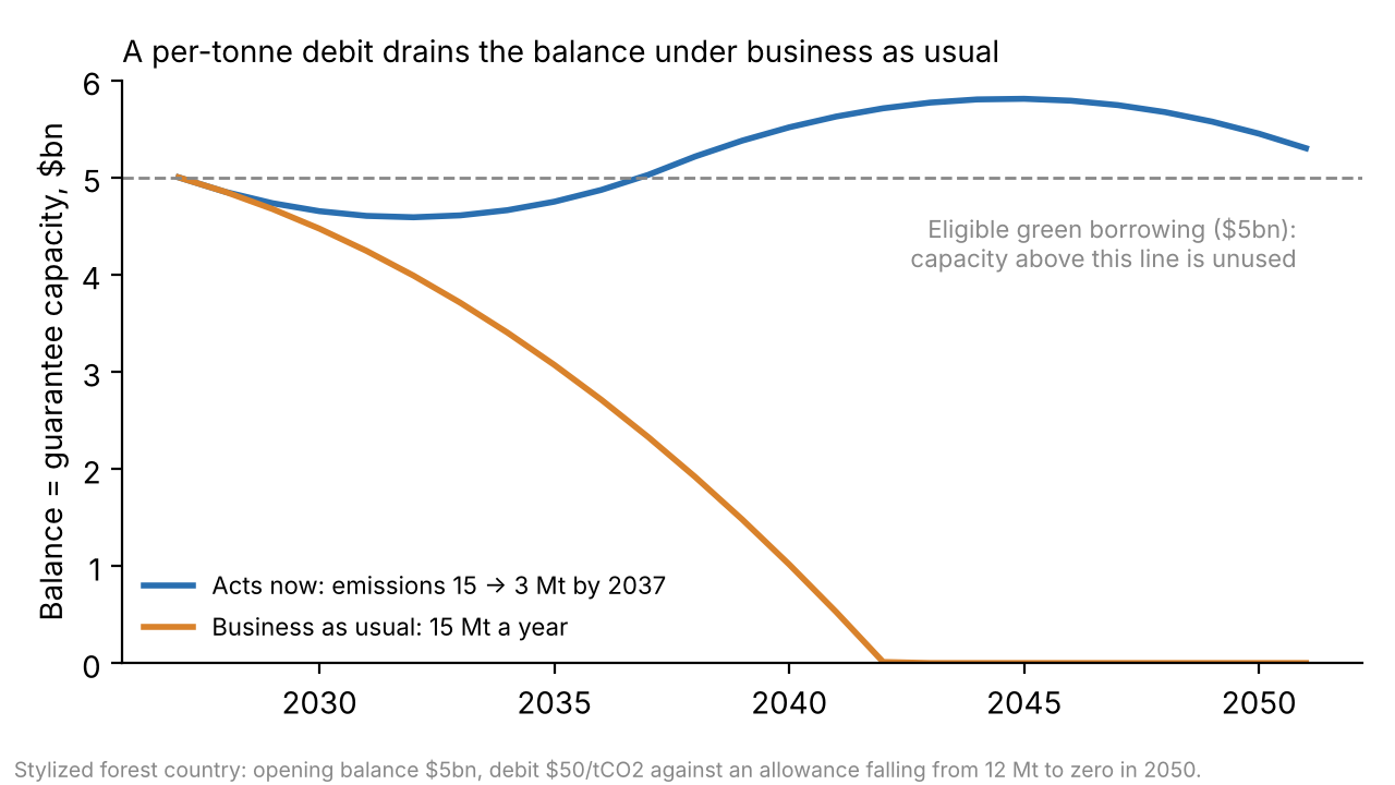
Business as usual drains the balance; action keeps it. Under business as usual the debit grows as the allowance falls, and the balance is exhausted in 2042 (Figure 1). A country that cuts emissions from 15 to 3 Mt by 2037 keeps its balance near its borrowing need throughout. The present value of spread savings over 2027–2050 is $2.11 billion if the country acts and $1.13 billion if it does not; acting is worth about $1 billion to it. From 2037 the acting country’s balance exceeds its $5 billion borrowing need, and by Proposition 2(d) a further tonne would then cost it nothing unless the surplus flows into a beneficiary account. That is why the surplus rule is part of the design, not an option.
Comparison with existing instruments. Table 4 puts the scheme beside the Guyana–Hess sale and the TFFF, converting each to a price per tonne at Guyana’s average carbon density. The TFFF’s $4 per hectare a year is about $0.004 per tonne of stock a year, equivalent to a stock price of $0.07 per tonne capitalized at 5 percent, under a third of the stock price used here. Its deforestation deduction of $400–800 per hectare is $0.37–0.74 per tonne released. The Hess price pays for avoided flow against a reference level and only for the credits sold. The NCV at a $50 debit price gives the stock a balance of the same order as the TFFF’s capitalized value and prices each tonne released at 40–80 times the TFFF’s deduction.
| Instrument | What is rewarded | Annual value to country | Price of a tonne released |
|---|---|---|---|
| Guyana–Hess ART-TREES sale (vintages 2016–2030) | Avoided emissions below an HFLD crediting level | About $50m (at least $750m for 37.5m credits) | $15–20 for credits sold |
| TFFF at $4/ha (Guyana-scale forest) | Standing forest area | About $72m | $0.37–0.74 (deduction per hectare ÷ density) |
| NCV, $5bn capacity, $50 debit (stylized) | Stock (opening balance) and every tonne emitted | $150m in spread saved | About $30 |
Two cautions apply. Guyana itself may be an awkward case for a guarantee-based reward: with large oil revenues, its need for guaranteed borrowing may be small relative to its stock, and for such a country the interest-on-balance variant is the better form (Section 7). And average density hides wide variation: a hectare of peat swamp or old-growth forest holds far more than a degraded one, so the debit per hectare cleared should use measured, not average, density.
6.4 How big must the scheme be?
The incentive scales with guaranteed borrowing, not with the stock. Proposition 1 makes the arithmetic linear: at a 3 percent saving, each $1 billion a year of incentive needs $33 billion of outstanding guarantee capacity. On the MDB record that capacity needs a buffer of $0.16 billion and costs donors about $13 million a year in expected losses; in the stress case the buffer is $3.1 billion and the cost $370 million (Table 5).
| Incentive to the country | Guarantee capacity needed | Buffer held: base (stress) | Expected donor cost a year: base (stress) | Present value of incentive over 20 years |
|---|---|---|---|---|
| $0.1bn a year | $3bn | $0.02bn ($0.3bn) | $1.3m ($37m) | $1.2bn |
| $0.5bn a year | $17bn | $0.08bn ($1.6bn) | $6.3m ($185m) | $6.2bn |
| $1bn a year | $33bn | $0.16bn ($3.1bn) | $12.6m ($370m) | $12.5bn |
| $5bn a year | $167bn | $0.8bn ($15.5bn) | $63m ($1.85bn) | $62bn |
These numbers explain why the guarantee form matters. The largest sovereign sustainability-linked loan to date, Uruguay’s $350 million World Bank loan of 2023, can save the country at most about $12.5 million over its life (Stretton 2026a). Multilateral REDD+ funds pledged about $6.4 billion from 2008, about $400 million a year (Government of Brazil 2025), so a results-based payment of $1 billion a year would be more than twice their average. A guarantee scheme delivering $1 billion a year of spread savings needs donors to accept about $13 million a year of expected losses on the MDB record, and about $370 million in the stress case. The buffer, $0.16 billion on the record and $3.1 billion in the stress case, is capital donors keep and which earns. Holding it is the job of the Climate Investment Trust (Stretton 2026g, 2026h).
The binding constraint is borrowing, not donor money. A country can only save spread on debt it actually issues, so the scheme delivers big incentives to countries that borrow a lot at high spreads: large, lower-rated forest and coal countries. For small or lightly indebted countries, the ceiling on the guarantee form is low, and the interest-on-balance variant or a link to the trust’s accounts must carry the reward.
6.5 A coal-reserve country
Fossil reserves raise the same question from the supply side: should a country be rewarded for coal it leaves in the ground? Indonesia had 34.9 billion tonnes of proved coal reserves at the end of 2020 (BP 2021), about 78 billion tonnes of CO₂ at IPCC default carbon contents (IPCC 2006). Valuing the whole reserve even at $1 per tonne would open a balance of $78 billion, and would reward the country for owning coal rather than for keeping it unburned.
Crediting the whole reserve would be a mistake. It rewards the largest fossil holders most, invites countries to report larger reserves, and pays for coal that would never be mined at today’s prices. The right base is narrower: credit only reserves that are legally and verifiably retired, by canceling concessions or mining licenses, and debit combustion emissions at the debit price as for any other country. Retiring 2 billion tonnes of bituminous coal, about 4.9 billion tonnes of CO₂, at a stock price of $1 per tonne would open $4.9 billion of capacity.
What that capacity is worth depends on the spread. For an investment-grade sovereign saving 1 percentage point, it is worth $49 million a year and each $1 of debit price converts to only 20 cents of carbon price; at a 3-point saving it would be worth $146 million a year. Guarantees are a strong incentive for countries that borrow at high spreads and a weak one for investment-grade emitters. For the latter, the same balance is better delivered as access to the trust’s collateral, or as a reward linked to sustainability-linked lending (Stretton 2026a).
Supply-side credits also leak. Retiring Indonesian reserves raises the world coal price and draws supply from elsewhere, so the emissions avoided are smaller than the carbon in the reserves retired (Harstad 2012). The debit on combustion emissions does not leak in this way, because it prices what the country burns. A coal country’s reward should therefore come mainly from the debit on its own emissions, with reserve retirement credited at a low stock price to reflect leakage.
6.6 Early action in numbers
Take a stylized energy reform: retiring coal capacity and replacing it with renewables at a net up-front cost of $1 billion, falling 5 percent a year as technology improves, cutting emissions by 5 MtCO₂ a year, with no domestic co-benefit counted and no ongoing cost. The minimum initial incentive from equation 9 is \((0.05 + 0.05) \times \$1\text{bn} / 5\text{ Mt} = \$20\) per tonne; with the option-value factor of 1.6–1.9 it is $32–37 per tonne. Below that level the government gains by waiting, and without any incentive it never acts (Figure 2). Counting a co-benefit of $5 per tonne, it would act without an incentive, but only after about 28 years.
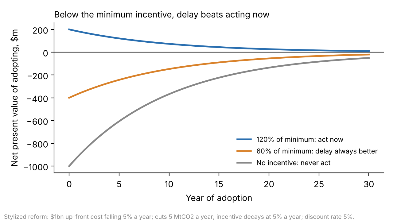
The decaying schedule halves the donor cost. To give $20 per tonne at the start with capacity that does not decline needs a debit price of $33 per tonne and costs donors $25 million in present value on the MDB record ($740 million in the stress case). With capacity declining at 5 percent a year, matching the fall in technology costs, the debit price must be $67 per tonne to deliver the same $20 at the start, but donors’ present-value cost falls to $13 million ($370 million in the stress case), because the incentive is concentrated where it changes the decision. Delivered as cash on results, the same incentive would cost $1 billion.
6.7 Sensitivity
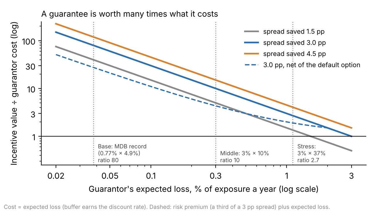
The ratio of value to cost is most sensitive to the spread saved, to whether the guarantor keeps preferred-creditor treatment, and to whether MDB capital is charged (Figure 3). Halving the spread to 1.5 points halves the budget ratio, to 40 in the base case and 1.4 in the stress case. Losing preferred-creditor treatment moves it from 80 toward 10 or 2.7; that is the main risk to the scheme’s cost, and the reason the stress case is reported throughout. Counting only the economic gain lowers it to about 27, and to 1.9 in the stress case, where a guarantee is barely better than a grant. If the guarantees were instead carried on an MDB balance sheet that holds capital at IBRD’s minimum equity-to-loans ratio of 18 percent (World Bank 2024), at a 2 percent carry, the base-case budget ratio would be about 7.5: still well above one, but a tenth of the headline. That is the case for holding a dedicated buffer in a trust rather than consuming MDB capital. The carbon-price equivalent is proportional to the debit price and the spread and inversely proportional to the discount rate plus decay, so a country with a 4.5-point spread gets half as much again per tonne as one with 3 points. On the budget measure, the guarantee form delivers more incentive per donor dollar than a grant unless expected losses exceed the spread saved, 3 percent a year, nearly 80 times the MDB record and almost three times the stress case.
7 Institutional delivery
MDBs issue the guarantees; a buffer fund stands behind them. The guarantees are ordinary MDB instruments: policy-based or project guarantees on the country’s eligible green borrowing, with a sovereign counter-indemnity. The NCV adds a rule for how much capacity each country gets, outside its normal lending envelope. The buffer that absorbs losses before they reach MDB capital is held by a fund that keeps capital rather than spending it; the Climate Investment Trust proposed in the companion paper is that fund (Stretton 2026g, 2026h). Holding capital rather than disbursing it is where the leverage comes from: even sized to the stress case, a buffer supports exposure about ten times its size. A call needs cash before recoveries arrive, so the fund also needs a liquidity line from its highly rated backer; if each call had to be paid from the buffer at a year’s debt service, $5 billion on the record would support about $390 billion of guarantees rather than about $1 trillion (Stretton 2026h).
Eligible borrowing must be defined narrowly. Capacity should cover borrowing for investments that cut emissions or protect stocks: clean power, grids, forest enforcement and monitoring, and the payment guarantees that make power purchase agreements bankable. Guarantee capacity earned under the NCV can stand behind the guarantee waterfall of the payment intermediary in Stretton (2026d) or the senior bonds of the asset-class structure in Stretton (2026c). Those papers report their own ratios, for example a contract guarantee that saves about $2 of tariff per dollar of expected cost in 3.1; that is a different quantity from Proposition 1, a guarantee on a utility’s payments to generators rather than on a sovereign’s debt, and the two should not be compared directly.
Interest on the balance, into a trust account, is the variant for non-borrowers. For a country that does not borrow enough for capacity to bind, the arrangement pays interest at rate \(i\) on the balance into a beneficiary account in the Climate Investment Trust, pledgeable as collateral now and withdrawable after 2050. The marginal incentive per tonne becomes \(p_e\, i/(r+\theta)\) in place of \(p_e \Delta s/(r+\theta)\), and the donor cost is the full interest, deferred, rather than a fraction of it. Surplus balance above a borrower’s capacity need flows into the same account, so the debit never goes slack.
Sustainability-linked lending is the delivery channel for the performance link. The debit and the allowance can be written as key performance indicators in a sustainability-linked loan or bond, so that meeting the allowance path both preserves the balance and triggers a step-down in the loan’s margin. Codified indicators and verification make that link routine (Stretton 2026a).
Verification uses existing systems. Forest stocks and land-use emissions can be measured under jurisdictional standards such as ART-TREES, which already verify national forest areas and emissions (Aster Global Environmental Solutions 2022); fossil emissions come from national inventories under the Paris transparency framework. The NCV needs these measurements annually, not a new market.
8 Risks and safeguards
Moral hazard: the guarantee makes the country borrow more. Cheaper borrowing invites more borrowing, and a guaranteed creditor has less reason to discipline the sovereign. Three features limit this. Capacity is capped by the balance, so the exposure is bounded. Only eligible green borrowing is covered. And the sovereign counter-indemnifies the guarantor, so a call on the guarantee becomes a debt to an MDB that the country has strong reasons to repay. The safeguard fails if eligibility is defined loosely or if the counter-indemnity is waived for the weakest borrowers, which is where the spread saved is largest.
Hidden fiscal exposure and subordination of other creditors. The scheme does not remove the host government’s liabilities. It converts part of its market debt into debt guaranteed by an MDB and backed by the government’s own counter-indemnity: the exposure becomes smaller in expected cost, contingent and contracted, but it is still the government’s. Because the guaranteed debt is in effect senior, the government’s other creditors stand further back in a default and may charge more, as Chamon et al. (2022) find for debt-for-climate swaps; part of the budget saving on guaranteed debt is then paid back on the rest. Proposition 1(b) gives the floor on the net gain. On the donor side, guarantee exposure is a contingent liability that capital-adequacy rules must count. A buffer sized to expected loss alone is used but not used up in normal years and is exhausted in a correlated crisis (Stretton 2026j, ch. 14); the buffer must be sized to stressed losses and its size published.
Valuation disputes. Countries will contest stock measurements, densities, allowances and the price. Separating the two prices narrows the stakes. Disputes over the stock and the allowance affect only the level of the balance, which is a matter of distribution and can be settled by negotiation (Proposition 2(c)). The debit price, which governs incentives, should be uniform across countries and set by rule. Prioritizing forests near ecological thresholds, where losing more forest could trigger dieback of much of the remainder (Lovejoy and Nobre 2018), is better done through a higher debit per hectare in designated zones than through a higher stock value, because the purpose is to price the next hectare cleared, not the hectares already standing.
Permanence and leakage. A forest can burn or be cleared after a contract ends. The NCV handles reversal by construction: a tonne released is debited whenever it is released, so a country cannot bank a reward and then reverse, provided the scheme is open-ended (Section 5.3). Natural disturbance needs a rule, such as a pooled insurance reserve, so that a fire beyond the government’s control does not wipe out a balance; the TFFF’s lower deduction for fire-degraded forest is a precedent (Government of Brazil 2025). Leakage within a country is avoided by national accounting; leakage across borders, as deforestation or coal supply moves to non-participants, is limited only by broad participation, which is an argument for opening the scheme to all forest and coal countries at once, as the TFFF does for 74 forest countries (Barber et al. 2025).
Fairness to low-stock countries. A stock-based balance gives most to countries with large forests and nothing to the Sahel or small island states. This is partly the point, since stocks are what a flow-based scheme fails to reward, but it cannot be the whole design. The allowance is the corrective: a low-emitting country with little stock earns balance every year it emits below its allowance, at the same debit price. A per-capita floor on the opening balance would add a further corrective. Because the incentive scales with borrowing, low-stock, low-borrowing countries are better served by the interest-on-balance variant than by guarantees.
The strongest objection: this pays for stocks that were never at risk, and invites hold-up. Much of Guyana’s or the Congo Basin’s forest is remote and would stand without any payment, so the opening balance is in large part a transfer for nothing; and paying for stocks, Harstad (2016) warns, rewards whoever threatens them most credibly. The answer has four parts. First, the transfer is infra-marginal by design, and it is cheap: what the country receives is capacity, costed to donors at expected loss plus buffer carry, not cash. Second, the opening balance is what makes the per-tonne debit enforceable; without a balance to lose, a sovereign cannot be charged for emitting. Third, by Proposition 2 the incentive at the margin is set by the debit price, not by the opening balance, so a generous stock credit does not dilute the incentive. Fourth, the balance is fixed at entry from a verified stock and the debit price is uniform, so a threat to clear raises neither; the alternative already in use, an HFLD adjustment to a crediting baseline, rewards the stock through exactly the counterfactual a threat can inflate. The objection is right that the stock price should be low. It is wrong that the stock should not be rewarded at all.
9 Policy implications
MDB shareholders should create a rules-based guarantee capacity outside country lending envelopes, allocated by notional capitalized value. Each participating country would receive an opening balance from its verified carbon stock at a low, uniform stock price, an allowance path to net zero, and a uniform debit price of $30–70 per tonne for emissions above the allowance, a carbon-price equivalent of about $18–42 at a 3-point spread. Capacity should be sized so that it binds on each country’s eligible green borrowing, decline at roughly the rate that clean technology costs fall, have no fixed end date, and pass any surplus to a beneficiary account.
Donors should fund the buffer rather than the reward. The first-loss buffer behind the guarantees should be held in a trust that invests it, sized to stressed losses on the exposure and published. On the calibration here, a scheme delivering $1 billion a year of incentive costs about $13 million a year in expected losses on the MDB record, and about $370 million in the stress case in which the facility does not inherit preferred-creditor status. Because the buffer is held rather than spent, donors should hold the stress-case buffer, about $3.1 billion, until the facility has a loss record of its own, with a liquidity line to pay calls before recoveries arrive. If holding it costs 2 percent a year, that adds about $62 million a year to the expected loss. Donors should present the budget saving and the economic gain together, so that host governments and parliaments see both.
Forest and coal countries should negotiate allowances, not baselines. Under the NCV the allowance affects how much a country gets, not how strongly it is rewarded per tonne, so it is a safer object of negotiation than a crediting baseline. Coal countries should seek credit for legally retired reserves at a low stock price, and should expect most of their reward to come from the debit on combustion emissions.
The scheme fails under five conditions. It fails if spreads saved are small, as for investment-grade sovereigns, unless the reward is delivered through the trust’s accounts instead. It fails if capacity is set so large that it never binds, which is the trap in the original proposal’s release schedule, or if the scheme has a fixed end date, which drains the price per tonne as the date approaches. It fails if the buffer is sized to expected rather than stressed losses, so that a correlated crisis reaches MDB capital. And it fails if verification is captured, so that measured emissions stop tracking real ones.
10 Conclusion
A notional capitalized value lets the international system reward what countries have kept as well as what they cut, at a fraction of the cost of paying for either in cash. Two results do most of the work. A guarantee saves the borrower the full spread and costs the provider only its expected loss and the carry on a buffer, so each dollar of expected loss buys about 80 dollars of interest saving on the MDBs’ own sovereign loss record and about 27 dollars of economic gain once the default option the country gives up is netted out; in a stress case without preferred-creditor status the figures are 2.7 and 1.9. And the stock and the margin need different prices: the stock opens the balance from which each tonne is debited, and the debit price, converted at the spread over the discount rate, sets the carbon-price equivalent. The main limitation is that the incentive scales with what a country borrows and the spread it saves, so the guarantee form is strong for large, lower-rated emitters and forest countries and weak for investment-grade or lightly indebted ones. The next step is to estimate spreads saved, risk premiums and eligible borrowing country by country, and to test with the companion trust model how large a buffer stressed, correlated losses require.
Downloads
References
Appendix A: Proofs
Proof of Proposition 1. (a) With constant parameters, equation 3 and equation 4 give \(V = (\Delta s - f)\sum_t \delta^t X_t\) and \(C = (\pi L + k\varphi - f)\sum_t \delta^t X_t\). The common factor \(\sum_t \delta^t X_t > 0\) cancels, giving equation 5. \(R > 1\) if and only if \(\Delta s - f > \pi L + k\varphi - f\), that is \(\Delta s > \pi L + k\varphi\), provided \(\pi L + k\varphi - f > 0\). With \(f = \pi L + k\varphi\), \(C = 0\) and \(V = (\Delta s - \pi L - k\varphi)\sum_t \delta^t X_t\).
- Per dollar of exposure a year, write the market spread as \(\Delta s = \ell_m + \rho\), where \(\ell_m\) is the market’s expected default loss and \(\rho\) the risk premium. Under market debt the country’s expected payment above the guaranteed rate is \(\Delta s - \ell_m\), because in default it does not repay what creditors lose. Under the guarantee it pays the guaranteed rate plus the fee; in default the guarantor pays creditors the expected shortfall \(\ell_m\), and the country repays the guarantor all of it except the guarantor’s own loss, \(\ell_m - \pi L\). Its expected payment above the guaranteed rate is therefore \(f - \ell_m + (\ell_m - \pi L) = f - \pi L\). The difference is \((\Delta s - \ell_m) - (f - \pi L) = \rho + \pi L - f\). Dividing by the guarantor’s cost \(\pi L + k\varphi - f\) and cancelling \(\sum_t \delta^t X_t\) as in (a) gives equation 6. Since \(\ell_m \ge \pi L\) when the guarantor is senior to market creditors, \(\rho + \pi L \le \Delta s\) and \(R_e \le R\). \(\square\)
Proof of Proposition 2. (a) In continuous time, \(\dot B_t = p_e(A_t - E_t)\), so emitting one extra tonne at \(s\) lowers \(B_t\) by \(p_e\) for all \(t > s\) (until the balance hits zero). Where capacity binds, \(X_t = \lambda_t B_t\), so guaranteed exposure falls by \(\lambda_t p_e\) and the country loses \((\Delta s - f)\lambda_t p_e\) a year. The present value at \(s\) is \[\int_s^\infty (\Delta s - f)\, p_e\, \lambda_0 e^{-\theta t} e^{-r(t-s)}\,dt = \frac{\lambda_0 p_e (\Delta s - f)}{r+\theta} e^{-\theta s}.\] If the scheme ends at \(\bar T\), the upper limit is \(\bar T\) and the value is multiplied by \(1 - e^{-(r+\theta)(\bar T - s)}\), which goes to zero as \(s \to \bar T\). (b) If the debit is \(p_e(A_t - \hat E_t)\) with \(\hat E_t\) a forecast fixed in advance, \(B_t\) does not depend on actual \(E_t\), so \(\partial V/\partial E_s = 0\). (c) \(A_t\) enters \(B_t\) additively and does not depend on \(E_s\), so \(\partial^2 B_t/\partial A\,\partial E_s = 0\) and \(\tau(s)\) is unchanged. (d) If \(\lambda_t B_t \ge D_t\), then \(X_t = D_t\) is locally unaffected by a small change in \(B_t\); if \(B_t = 0\), the floor in equation 1 makes \(B_t\) locally insensitive to further emissions. In either case the integrand is zero for those \(t\). \(\square\)
Proof of Proposition 3. Differentiate equation 8: \(W'(T) = -\Delta E\,[m(T) + b - \omega]e^{-rT} + (r+g)K_0 e^{-(r+g)T}\). Multiply by \(e^{(r+g)T} > 0\): the sign of \(W'(T)\) is the sign of \(h(T) \equiv (r+g)K_0 - \Delta E\,n(T)e^{gT}\), where \(n(T) = m(T) + b - \omega = (m_\infty + b - \omega) + (m_0 - m_\infty)e^{-\theta T}\). Then \(n(T)e^{gT} = (m_\infty + b - \omega)e^{gT} + (m_0 - m_\infty)e^{(g-\theta)T}\). The first term is non-decreasing because \(m_\infty + b - \omega \ge 0\) (persistence), and the second is non-decreasing because \(\theta \le g\) and \(m_0 \ge m_\infty\). So \(h(T)\) is non-increasing. If equation 9 holds, \(h(0) \le 0\), so \(h(T) \le 0\) and \(W'(T) \le 0\) for all \(T \ge 0\): \(W\) is non-increasing and \(T = 0\) is optimal. Since \(W(T) \to 0\) as \(T \to \infty\), also \(W(0) \ge 0\), so acting now beats never acting. Conversely, if equation 9 fails, \(h(0) > 0\), so \(W'(0) > 0\) and adopting slightly later beats adopting now.
For the cost result, the donors’ present-value cost of incentives for abatement \(\Delta E\) from \(T = 0\) is \(\frac{\pi L + k\varphi}{\Delta s}\int_0^\infty \Delta E\,m(s)e^{-rs}\,ds = \frac{\pi L + k\varphi}{\Delta s}\Delta E\left[\frac{m_\infty}{r} + \frac{m_0 - m_\infty}{r+\theta}\right]\), which is decreasing in \(\theta\) for \(m_0 > m_\infty\). Under the sufficient condition \(\theta \le g\), the cost is minimized at \(\theta = g\), with \(m_0 = m_0^*\) and \(m_\infty\) at its lowest permitted value \(\max(\omega - b, 0)\). \(\square\)
Remark 1 (no incentive). With \(m \equiv 0\), \(h(T) = (r+g)K_0 - \Delta E(b-\omega)e^{gT}\). If \(b \le \omega\), \(h > 0\) for all \(T\) and the government never acts. If \(b > \omega\), \(h\) falls and crosses zero at \(T^* = \tfrac1g \ln[(r+g)K_0/(\Delta E(b-\omega))]\), the optimal adoption date.
Remark 2. For \(\theta > g\), equation 9 remains necessary but is no longer sufficient: \(h(T)\) may rise and then fall, and a later adoption date can dominate. The code in Appendix B checks \(W(T)\) numerically for any schedule.
Appendix B: Data and code
All calculations are in 2.Source/model.py, which prints every number used in the paper and the brief; 2.Source/make_wp_figures.py draws the three figures. Both run with Python 3, NumPy and Matplotlib.
Anchored data. Guyana’s forest carbon stock (19.5 GtCO₂e) and forest area (about 18 million hectares) are from Government of Guyana (2022). The Hess sale terms and the ART issuance are from Department of Public Information, Guyana (2023), and Guyana’s HFLD crediting level from Aster Global Environmental Solutions (2022). TFFF design figures are from the facility’s official Concept Note 3.0 (Government of Brazil 2025), and its launch, pledges and eligible countries from Barber et al. (2025). The base-case call probability and loss per call are the MDB default and recovery rates of European Investment Bank (2025); the middle and stress cases and the buffer sizes are those of Stretton (2026h), with the stress-case loss per call from Cruces and Trebesch (2013). The risk premium share is from Longstaff et al. (2011). IBRD’s equity-to-loans minimum is from World Bank (2024), and the Gabon bond terms from African Sovereign Debt Justice Network (2023) and Smith (2023). Indonesia’s coal reserves are from BP (2021); carbon contents use IPCC default net calorific values and emission factors for other bituminous coal (25.8 GJ/t, 94.6 kgCO₂/GJ, so 2.44 tCO₂/t) and sub-bituminous coal (18.9 GJ/t, 96.1 kgCO₂/GJ, so 1.82 tCO₂/t), the latter applied to lignite as well, which overstates its carbon (IPCC 2006).
Option-value factor. For a cost following a driftless geometric random walk with volatility \(\sigma\) and a deterministic benefit, \(\beta\) is the positive root of \(\tfrac12\sigma^2\beta(\beta-1) - r = 0\). At \(r\) = 5 percent, \(\sigma\) = 15 percent gives \(\beta\) = 2.67 and a factor of 1.60; \(\sigma\) = 20 percent gives \(\beta\) = 2.16 and 1.86.
Stylized inputs. Eligible green borrowing ($5 billion), the emissions and allowance paths, the debit price ($50 per tonne), the asset correlation (0.2) and number of programs (20) behind the buffer sizes, the middle and stress cases for guarantee losses (from the companion paper), the investment-grade spread (1 percentage point), the discount rate (5 percent) and the early-action reform (cost $1 billion falling 5 percent a year, 5 MtCO₂ a year cut) are assumptions for illustration.
Footnotes
The mechanism first appears as the Notional Capitalized Carbon Value in chapter 21 of the author’s book manuscript Time and Chance (Stretton 2026j), as a fallback in the Climate Investment Trust proposal (chapter 20 of the same book) and on the author’s research page. The forest-valuation argument draws on chapters 5–7 of Carbon Pricing: The Right Policy at the Wrong Time (Stretton 2026i). The three quantities of Section 5.5 come from the author’s DPhil research proposal (Stretton 2026f). All errors are the author’s.↩︎