Credit the Price Signal, Not the Payment
Carbon Price Recognition and Scrap Shuffling under the EU’s Carbon Border Adjustment Mechanism
The EU’s Carbon Border Adjustment Mechanism measures embodied carbon plant by plant and credits only carbon prices effectively paid. Both rules work against its second purpose, encouraging trading partners to decarbonize. A producer can send scrap-based steel to Europe and blast-furnace steel elsewhere, cutting its charge without cutting emissions. And a revenue-neutral feebate, which charges the full rate at the margin, earns nothing because its average payment is zero. I show that measuring embodied carbon by country and sector removes the gain from shuffling, that it leaves individual plants almost no incentive unless the exporting country prices carbon itself, and that crediting the country’s price signal supplies that incentive. A liability formula with this property is calibrated to the EU’s default values. At €80 per tonne, shuffling saves €98–626 per tonne of steel across thirteen exporters; recognizing the signal halves the share of output an exporter must sell to the EU before a feebate pays for itself. Full recognition has a cost: an exporter with a feebate at the EU price would pay no charge while EU producers pay on all their emissions. Recognition should therefore rise with the phase-out of free allocation, with relocation reviews.
carbon border adjustment, CBAM, carbon price recognition, feebates, resource shuffling, steel, default values
Working paper, version 0.4, October 2026. Stephen J. Stretton, writing in a personal capacity. The views expressed are the author’s own and do not represent those of any institution with which he is or has been affiliated. A short version for policy makers is Climate Fiscal Policy Brief No. 1.4. Legal texts are as of 31 October 2026; version 0.2 was the author’s submission to the Commission’s consultation of May–June 2026 (Stretton 2026a). All CBAM amounts are in euros.
1 Executive summary
Policy brief (short version) → · Download this paper (pdf) · Slides (pdf)
The EU’s border charge on carbon rewards the wrong things in its trading partners. Since January 2026, EU importers of steel, aluminum, cement, fertilizers, hydrogen and electricity owe certificates for the carbon embodied in what they buy. The Carbon Border Adjustment Mechanism (CBAM) is meant both to put imported and EU-made goods on an equal footing and to encourage exporting countries to cut their own emissions. Two of its rules serve the first purpose and work against the second. Embodied carbon is measured plant by plant. And the charge falls only by a carbon price “effectively paid” abroad, net of any rebate.
Plant-by-plant measurement pays exporters to reroute clean steel rather than to make cleaner steel. A steelmaker with blast furnaces and scrap-fed electric furnaces can send the scrap-based steel to Europe and sell the rest elsewhere. In a stylized exporter selling a tenth of its output to the EU, the carbon the border sees falls by 76 percent and the bill by €102 million a year, while the exporter’s emissions do not change. Across thirteen exporters, at €80 per tonne of CO₂, the gain is €98–626 per tonne of hot-rolled steel routed: €310 for India, €223 for China, €162 for Türkiye. Scrap is limited, so the reported cut is mostly relabeling.
Crediting only the price paid gives nothing to the instrument most likely to survive the politics of a large emitter. A revenue-neutral feebate charges each producer the carbon price on emissions per tonne above its sector’s average and rebates it below. Every producer faces the full price on each tonne it cuts, but the average producer pays nothing, so under the Commission’s draft rules the feebate earns no credit. A carbon tax at the same rate, which produces the same cuts, would earn the whole of it.
Measuring by country and sector removes shuffling, but by itself it leaves plants with almost no reason to cut. If every tonne from a country is charged at the sector’s average, routing earns nothing. But a single plant that cleans up lowers the average for all its country’s exporters, so it keeps only a sliver of the reward. That is why the two fixes belong together: a domestic feebate gives every plant the full incentive on all its output, and recognizing the feebate at the border rewards the country for adopting it.
I propose that the liability on imports be the EU price less a recognized foreign price, times the country-sector average carbon content. The recognized price is the price paid plus a weight on the part of the country’s price signal that is not paid. This rule does not depend on which plant ships the goods, and it keeps the exporter’s lowest-cost feebate rate at the EU’s own price. Opting into this rule with a feebate at €80 removes India’s €445 per tonne liability on hot-rolled steel; under today’s rules the feebate earns no credit at all. Recognition also changes what an exporting country would choose for itself. If it sells a tenth of its steel to the EU, its own best feebate rate rises from €8 to €21; a feebate at the EU price pays for itself once more than 24 percent of output goes to the EU, against half under today’s rules.
The cost is a weaker level playing field, which is why recognition should be phased in. An exporter with a feebate at the EU price would pay no border charge while EU producers pay on all their emissions once free allocation ends. Recognition should therefore rise in step with the phase-out of free allocation to EU producers, now due by 2034 and possibly 2038, with a review of relocation before each step.
What to do. The Commission should consult on its default carbon price methodology, now in preparation, and let it cover feebates and other instruments measured as carbon-price equivalents; offer country-sector values without the mark-up to countries with a recognized price signal; and measure shuffling from installation-level declarations. Exporting countries should consider a sector-wide feebate.
2 Introduction
The EU’s Carbon Border Adjustment Mechanism (CBAM) is the first border charge on embodied carbon at scale, and its design choices will shape which carbon-pricing instruments its trading partners adopt. Since January 2026 importers of iron and steel, aluminum, cement, fertilizers, hydrogen and electricity have owed certificates for the emissions embodied in what they import, priced in line with the EU Emissions Trading System and on sale from February 2027 (European Parliament and Council of the European Union 2023b, 2025). Free allocation to EU producers in the same sectors is phased out as the charge is phased in, by 2034 under current law (European Parliament and Council of the European Union 2023a) and by 2038 under a Commission proposal of July 2026 (European Commission 2026b). At €80 per tonne of carbon dioxide and full phase-in, the charge on a tonne of hot-rolled steel from India, declared at the Commission’s default value with its 30 percent mark-up, is €445; from China, €331; from Türkiye, €252 (Section 8).
The mechanism has two purposes. The first is a level playing field: an imported tonne of steel should bear the same carbon cost as a tonne made in the EU, and no tonne should be charged twice. The second is to encourage the countries that export to Europe to decarbonize their own production. Two rules serve the first purpose well and the second badly. Embodied carbon is measured plant by plant, from verified installation data or from a country default value. And the charge falls only by a carbon price “effectively paid” in the country of production, taking into account “any rebate or other form of compensation” (European Parliament and Council of the European Union 2025, Art. 9(1)).
Each rule creates a flaw. Plant-level measurement lets an exporter with both blast furnaces and scrap-based electric arc furnaces route the scrap-based steel to Europe and the rest elsewhere, cutting the carbon the border sees without cutting the carbon in the atmosphere. Price-paid recognition credits payments, not incentives: a revenue-neutral feebate charges every producer the full rate on each tonne above a sector benchmark and rebates the rest, so it sends the full price signal while its average producer pays nothing. The Commission’s draft rules on the carbon price paid treat emissions “below an emission intensity baseline” as compensation to be netted off (European Commission 2026a, Art. 8(1)(b)(ii)), so the feebate earns nothing.
The question this paper answers is how CBAM should measure embodied carbon and foreign carbon prices so that it rewards decarbonization rather than routing. The answer is to measure both by exporting country and sector, and to credit the foreign price signal, the marginal cost a country’s instruments put on emitting, alongside the price paid. Country-sector measurement does not depend on which plant shipped the goods, so routing earns nothing. On its own it leaves each plant almost no incentive, because a plant that cleans up lowers the average for all its country’s exporters. A domestic feebate restores the incentive on every tonne the country makes, and crediting it gives the country a reason to adopt it. The Total Effective Carbon Price of paper 6.1 (Stretton 2026d) supplies the measure, for price and non-price instruments alike.
The paper makes four contributions, each against named prior work.
- A model of route shuffling (Section 5). Mehling and Ritz (2023) identify the trade-off between default and actual intensities and the risk of reshuffling, but do not model it. Under plant-level measurement an exporter sends its low-carbon output to the EU up to its capacity or its EU sales, whichever binds, and its bill falls by \(\tau(e_B - e_S)\) per tonne routed with no change in its emissions (Proposition 1). When scrap is scarce, world emissions do not change either (Proposition 2). Under country-sector measurement routing earns nothing, but a plant’s own reward for cutting intensity is its firm’s EU share of the sector’s output, close to zero (Proposition 3). That is the property Neuhoff et al. (2026) concede for their standardized values, which “would not create direct incentives” abroad.
- A liability formula (Section 6). Mehling and Ritz (2023) write the border charge as a top-up on the shortfall of the foreign explicit carbon price and say it does not attempt to include “effective” prices. A feebate earns nothing under price-paid recognition (Proposition 4). I propose certificates on \((\tau - r)^{+}\) per tonne of embodied carbon measured at the verified country-sector average, where the recognized price \(r\) adds a weight \(\rho\) on the unpaid part of the price signal. The liability is invariant to shuffling, and with full recognition each exporter’s most competitive feebate rate equals the EU’s carbon price, as in Proposition 7 of the companion paper (Stretton 2026e) (Proposition 5).
- The verification trade-off (Section 7). Any rule that rewards a plant for verifying its own low intensity also rewards shipping from the cleanest plant, one for one (Proposition 6). I recommend a hybrid: country-sector measurement for countries with a recognized price signal, which then supplies the plant-level incentive itself, and firm-level verification of whole output, the remedy Mehling and Ritz (2023) suggest, for the rest.
- A calibration (Section 8) to the Commission’s default values for 119 countries. The shuffling gain is €98–626 per tonne of steel routed. Full recognition halves the share of a sector’s output that must go to the EU before a feebate at the EU price pays for itself, from one half to about a quarter.
The paper belongs to a series. Paper 1.1 sets out the two-track architecture, a production feebate and a destination-based consumption charge, and proves that a charge on embodied carbon measured by country and sector makes each exporter’s most competitive feebate rate equal to the charge (Stretton 2026e). Paper 1.2 designs feebates (Stretton 2026c); paper 6.1 measures any instrument as a carbon-price equivalent (Stretton 2026d). This paper applies them to the border mechanism that exists.
3 CBAM as legislated
CBAM rests on two measurements, and both are plant-level by default. The importer surrenders certificates equal to the embodied emissions of its imports, adjusted for the free allocation EU producers still receive, less a reduction for carbon prices paid abroad (European Parliament and Council of the European Union 2023b). Embodied emissions are declared either from actual values, verified by an accredited verifier at the installation, or from default values set by the Commission (European Parliament and Council of the European Union 2023b, Art. 7; European Commission 2025c, 2025b). For iron and steel and aluminum only direct emissions count (European Parliament and Council of the European Union 2023b, Annex II). Importers below a single threshold of 50 tonnes a year across these goods are exempt (European Parliament and Council of the European Union 2025, Annex VII). Table 1 lists the texts and their status.
| Text | Subject | Status at 31 October 2026 |
|---|---|---|
| Regulation (EU) 2023/956 | Establishes CBAM; definitive period from 1 January 2026 | In force; Article 9 replaced by 2025/2083 |
| Regulation (EU) 2025/2083 | Simplification: 50-tonne threshold; new Article 9 with yearly default carbon prices; default values at country averages plus mark-up | In force since October 2025 |
| Directive (EU) 2023/959 | Free allocation to CBAM sectors phased out 2026–2034 | In force; COM(2026) 616 would extend to 2038 |
| Implementing Regulation (EU) 2025/2621 | Default values by country and product, with mark-ups | Applies from 1 January 2026; to be revised in 2027 at the latest |
| Implementing Regulation (EU) 2025/2620 | Free-allocation adjustment, with benchmarks by production route | In force |
| Implementing Regulations (EU) 2025/2546 and 2025/2547 | Verification principles; methods for calculating embedded emissions | In force |
| Draft implementing regulation, Ares(2026)4841230 | Carbon price paid in a third country: conversion, evidence, independent persons | 177 responses to feedback; in adoption workflow; not adopted |
| COM(2025) 989 | Proposal: downstream goods, anti-circumvention, pre-consumer scrap | Pending in co-decision |
Default values are country averages with a penalty on top. Since the 2025 amendment, default values “shall be set at the average emission intensity of each exporting country … increased by a proportionately designed mark-up”; where reliable country data are lacking, at the average of the ten exporting countries with the highest intensities (European Parliament and Council of the European Union 2025, Annex IV point 4.1, recital 35). Implementing Regulation 2025/2621 sets the mark-up for iron and steel, aluminum and cement at 10 percent in 2026, 20 percent in 2027 and 30 percent from 2028, and 1 percent for fertilizers (European Commission 2025f). For hot-rolled flat steel (CN 7208), the defaults before mark-up are 4.28 tCO₂ per tonne for India, 3.19 for China and 2.43 for Türkiye, and 4.05 for countries without reliable data. Each country line also carries a production-route code that sets the benchmark for the free-allocation adjustment (European Commission 2025e). The mark-up has a job: a plant cleaner than its marked-up country default gains by filing verified data, so the mark-up draws data out of the cleaner plants. A plant dirtier than the default has no reason to file. The defaults are fixed by implementing act until their revision, due in 2027 at the latest (European Commission 2025f, Art. 2).
Article 9 credits payments, and only where a carbon price is set by rule. Under Article 9(1), as replaced in 2025, a declarant using actual emissions may claim a reduction “only if the carbon price has been effectively paid in a third country”, and “any rebate or other form of compensation available in that country that would have resulted in a reduction of that carbon price shall be taken into account” (European Parliament and Council of the European Union 2025). A declarant using default values may claim a reduction only by reference to yearly default carbon prices, and only “where a carbon price was set by the rules applicable in the third country and a yearly default carbon price can be determined, including on a conservative basis” (Art. 9(4)). “As from 2027, the Commission may, for third countries where carbon pricing rules are in place, determine and make available … the default carbon prices for those third countries and publish the methodology for their calculation”, using “the best available data”, and taking rebates and compensation into account (Art. 9(4); recital 20). Article 9(5) empowers the Commission to set by implementing act how prices paid and default prices convert into fewer certificates, what evidence is needed, and to give examples of rebates or compensation. “Carbon price” itself means “the monetary amount paid in a third country … in the form of a tax, levy or fee or in the form of emission allowances” (European Parliament and Council of the European Union 2023b, Art. 3(29)).
Three consequences follow for a typical developing-country exporter. First, the default carbon price is the only route open to an exporter that declares default values, which most will in the early years, and the law makes it discretionary and confines it to countries that already have carbon pricing rules. For a country whose carbon pricing consists of fuel excises or subsidy reform, the default is zero by construction. Second, the methodology is in preparation but not published: the Commission has contracted a consortium led by Technopolis Group to develop it, with default carbon price estimates for 2026 to 2028, starting from an inventory of emissions trading systems and carbon taxes assessed against eligibility criteria (Technopolis Group 2026). Nothing has been put out for consultation. Third, every recognition route nets out rebates.
The draft implementing regulation makes the netting explicit. The draft published for feedback on 13 May 2026 builds the price paid up good by good: only mechanisms that are “binding in nature” and impose compliance obligations on all operators in the sector count; their covered emissions are attributed to each good; and free allowances, exemptions, reduced rates, refunds and compensation are deducted (European Commission 2026a, recital 8, Arts. 6 and 8). Article 8(1)(b)(ii) counts as compensation the emissions “below an emission intensity baseline under a baseline-and-credit emissions trading system”. This is the provision behind the recognition flaw. Article 8(2) exempts subsidies financed from the mechanism’s revenues from netting if all installations are eligible whatever price each paid, support is granted on application by a public decision, and its objective is to cut the beneficiary’s emissions. The draft also caps international credits under Article 6 of the Paris Agreement at 10 percent of covered emissions. It drew 177 responses and, at 31 October 2026, was in the Commission’s adoption workflow, not adopted.
Shuffling is monitored but not prevented. Regulation 2023/956 asks the Commission to report from 2028 on the mechanism’s effect on “international trade, including resource shuffling” (European Parliament and Council of the European Union 2023b, Art. 30), but provides no enforcement (Assous et al. 2024). The Commission’s December 2025 proposal would add to the list of circumvention practices “artificially adjusting the supply chains of goods to benefit from lower default value”, and would bring pre-consumer scrap into scope as a precursor (European Commission 2025g). It does not touch routing between installations under actual values, which is the case modeled in Section 5.
4 Related literature
The paper joins four literatures at one point none of them addresses: how a border charge should recognize foreign policy when the foreign producer can choose which plant supplies the border. Appendix A reviews them in more detail.
Border carbon adjustment design. The design literature treats recognition of foreign effort as a choice and generally recommends crediting it (Ismer and Neuhoff 2007; Mehling et al. 2019; Cosbey et al. 2019; Kortum and Weisbach 2017; Keen et al. 2022). Keen et al. (2022) recommend starting from domestic benchmarks and moving to country values later. Clausing and Wolfram (2023) show that when some countries price carbon and others subsidize clean production, one border instrument cannot handle both; the feebate, which prices at the margin and subsidizes on average, sits between their two cases. The closest prior design is Mehling and Ritz (2023), who charge imports on the shortfall of the foreign explicit carbon price, \(\max\{t - t_k, 0\}\), times the lower of actual and default intensity, and leave “effective” prices aside. The closest alternative is Neuhoff et al. (2026), who propose standardized values independent of production process and location, with a standardized liability per tonne of material and export relief. Their design removes shuffling by construction and, they say, creates no direct incentive for producers abroad. This paper keeps their insight that the measure should not depend on which plant ships, and adds the missing incentive through the exporting country’s own instrument.
Measurement of embodied carbon and shuffling. Mehling and Ritz (2023) show that a border charge based only on default intensities removes the incentive to cut intensity, while one based on actual intensities restores it but opens resource shuffling. They judge shuffling likely to be smaller for industrial goods than for electricity, because material flows are easier to trace, and suggest regulating at company rather than installation level. The quantitative evidence is from electricity. In California, a cap-and-trade program without rules on imported power would leak 45 percent of its domestic reduction; with imports capped and shuffling banned, 9 percent (Caron et al. 2015). Exempting out-of-state generators achieves about a third of the reductions of complete regulation at more than twice the cost per tonne (Fowlie 2009). Bushnell et al. (2014) analyze the downstream regulation of imported power under California’s program. For CBAM, Assous et al. (2024) estimate that fees on imports from China would be €313 million a year under shuffling against €590 million with unchanged trade flows, at full phase-in; Apaydın (2026) finds that CBAM’s electricity-accounting rules let Chinese industrial parks report cuts that correspond to a fraction of real abatement; and the first data on steel trade under the definitive regime show no broad shift of EU flat-steel imports away from origins with high default values in January–June 2026 (Hamidani 2026). No study measures routing between plants within an exporter.
Measuring carbon prices beyond explicit ones. The World Bank’s total carbon price adds fuel excises net of subsidies to explicit prices for 142 countries; indirect pricing is “the lion’s share” of the world’s carbon price and matters most in developing net fuel importers (Agnolucci et al. 2024). The IMF benchmarks fuel prices against efficient levels that include environmental costs (Black et al. 2023), and the OECD publishes effective carbon rates (OECD 2023). These measure the average price per tonne. Paper 6.1 converts any instrument, including standards and feebates, into the uniform tax that cuts emissions as much (Stretton 2026d).
Intensity-based pricing. Output-based rebating, tradable performance standards and feebates price emissions intensity at the full rate while returning revenue in proportion to output (Fischer 2001; Fischer and Fox 2012; Holland et al. 2009). Hagem et al. (2020) show that refunding in proportion to abatement spending, the economic content of the draft’s Article 8(2), needs a lower fee than a tax for the same abatement.
The gap. The literature has a shuffling problem for electricity, a recognition rule for explicit prices, a measurement framework for non-price instruments and a standardized-value design that gives up foreign incentives, but no model of how plant-level measurement and price-paid recognition interact, no liability formula that handles both while keeping an incentive abroad, and no calibration to the default values now in law. The incidence literature shows why it matters: exposure relative to the size of the economy falls on middle- and low-income exporters with weak verification capacity (Eicke et al. 2021; Beaufils et al. 2023; Magacho et al. 2024; Perdana and Vielle 2022), and charges set on country averages fall hardest on poorer exporters (Mattoo et al. 2009).
5 A model of route shuffling
Setup. An exporter, a firm or a country’s steel sector, has two production routes: blast furnace with basic oxygen furnace (BF-BOF), at emissions intensity \(e_B\) tonnes of CO₂ per tonne of steel, and scrap-based electric arc furnace (scrap-EAF), at \(e_S < e_B\). Outputs are \(q_B \le K_B\) and \(q_S \le K_S\), total output \(Q = q_B + q_S\), and the scrap share \(s = q_S/Q\). The average intensity is \(\bar e = s e_S + (1-s) e_B\). The product is homogeneous. The exporter sells \(Q_{EU}\) to the EU, a share \(\mu = Q_{EU}/Q\), and the rest in markets without a carbon charge. It chooses \(x\), the scrap-route output sent to the EU, with \(0 \le x \le \min(q_S, Q_{EU})\); the remaining \(Q_{EU} - x\) comes from BF-BOF. The EU charges \(\tau\) per tonne of embodied CO₂, at full phase-in. Routing costs \(c\) per tonne moved away from proportional sourcing, \(x_0 = s\,Q_{EU}\).
Two measurement regimes are compared. Under plant-level measurement, the CBAM bill is \(\tau[e_S x + e_B (Q_{EU} - x)]\). Under country-sector measurement, every tonne from the exporter is charged at the verified sector average, \(\tau \bar e\, Q_{EU}\).
Proposition 1 (shuffling under plant-level measurement). Hold outputs fixed and let \(\tau(e_B - e_S) > c\). Under plant-level measurement the exporter sends \(x^* = \min(q_S, Q_{EU})\) of scrap-route steel to the EU. Relative to proportional sourcing its CBAM bill falls by \[ \Delta B = \tau\,(e_B - e_S)\,\big[\min(q_S, Q_{EU}) - s\,Q_{EU}\big], \tag{1}\] gross of routing costs, which equals \(\tau(\bar e - e_S)\,Q_{EU}\) when \(q_S \ge Q_{EU}\). Its total emissions \(e_B q_B + e_S q_S\) do not change. When \(q_S \ge Q_{EU}\), the CBAM gives no incentive to cut BF-BOF intensity.
The proof is in Appendix B. The bill is linear in \(x\) with slope \(-\tau(e_B - e_S)\), so the exporter fills EU orders from the scrap route until it runs out of scrap-route output or EU orders. The second form of equation 1 is useful for calibration: once scrap capacity covers EU sales, the gain depends only on the gap between the exporter’s average intensity, which the country default values estimate, and scrap-EAF intensity.
A worked example shows the magnitude (stylized). An exporter makes 10 Mt of crude steel a year: 8 Mt by BF-BOF at 2.0 tCO₂/t and 2 Mt by scrap-EAF at 0.4 tCO₂/t. The International Energy Agency gives 2.2 and 0.3 tCO₂/t for the two routes counting direct and indirect emissions, and 1.2 and 0.04 counting direct emissions only, because it books power made from steel-mill gases as indirect (International Energy Agency 2020, Box 1.3). The stylized gap between routes, 1.6 tCO₂/t, is smaller than the IEA’s 1.9, so the example understates the gain. The exporter emits 16.8 MtCO₂, 1.68 tCO₂/t on average, and sells 1 Mt to the EU at €80/tCO₂. Proportional sourcing puts 1.68 MtCO₂ on the EU’s books and a bill of €134 million. Sending scrap-EAF steel only puts 0.40 MtCO₂ there, 76 percent less, and a bill of €32 million. The saving, €102 million a year, is equation 1 with \(s = 0.2\). Emissions stay at 16.8 MtCO₂ (Figure 1).
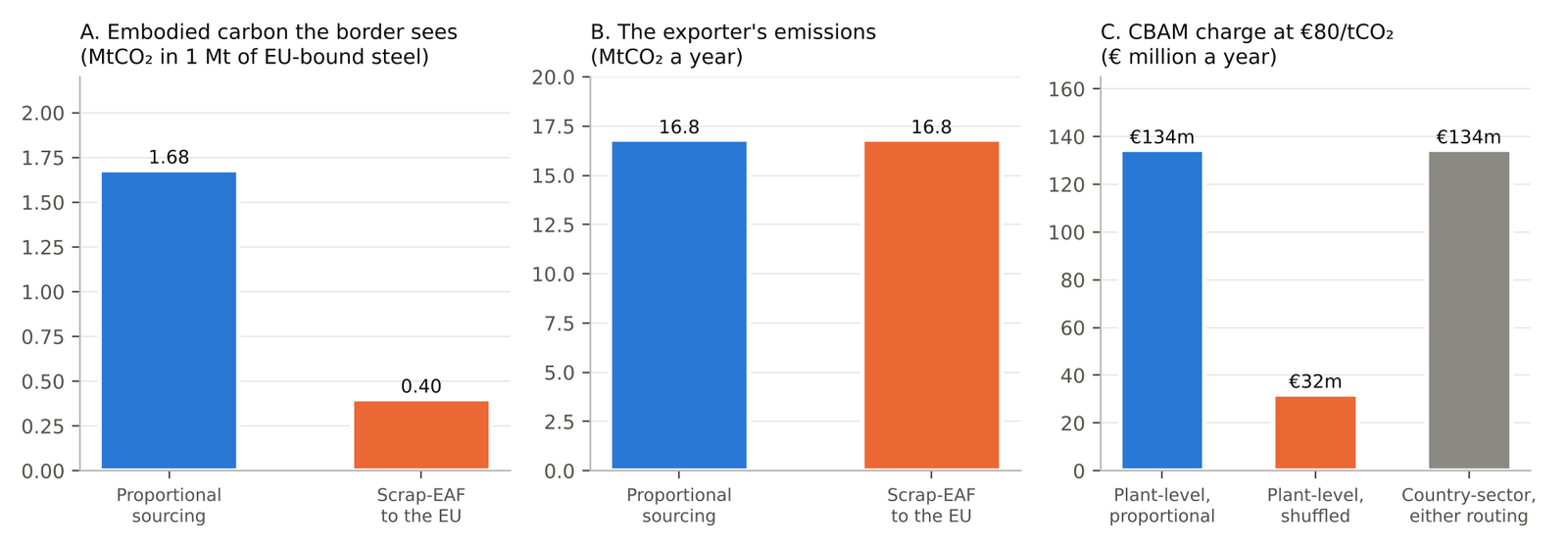
2.Source/make_wp_figures.py.
Firms do not need to coordinate for the result to hold at sector level. If the sector consists of separate BF-BOF and scrap-EAF firms, plant-level measurement creates a premium in the EU market for low-carbon steel of up to \(\tau(e_B - e_S)\) per tonne. Competitive sorting then sends scrap-EAF output to the EU first, exactly as a single firm would. World Bank analysts note the same pattern from the other side: firms that produce steel for export may have lower emissions than those producing for the domestic market (Maliszewska et al. 2025).
Default values open a second route to the same result. A plant may declare actual or default values. With verification free, plant \(i\) declares \(\min\{e_i, (1+m)\bar e_c\}\), where \(\bar e_c\) is the country default before mark-up \(m\). In a mixed-route country, scrap-EAF plants file actual data and BF-BOF plants dirtier than the marked-up default declare the default, so the declared intensity of EU-bound steel sits below the country average even with no routing. The mark-up narrows this selection but does not close it, and the anti-circumvention clause of COM(2025) 989, aimed at supply chains adjusted to reach lower default values, does not reach it (European Commission 2025g).
Scrap is scarce, so the low intensity of scrap-based steel is largely borrowed. Steel scrap is a by-product of past steel use: its availability “is finite and predetermined”, set by the rate at which steel products reach the end of their life and by collection and sorting, with a cost curve that brings out more at higher prices (International Energy Agency 2020, 28–30). Suppose the exporter expands scrap-EAF output by \(\Delta\) to serve the EU, global scrap collection rises by \(\theta\Delta\) with \(0 \le \theta \le 1\), and the users from whom the remaining scrap is diverted replace it with steel at intensity \(e_R\).
Proposition 2 (world emissions with scarce scrap). Reported embodied carbon in EU imports falls by \((e_B - e_S)\Delta\). World emissions change by \(-(e_B - e_S)\Delta + (1-\theta)(e_R - e_S)\Delta\), which is \(-\theta(e_B - e_S)\Delta\) when displaced users turn to blast-furnace steel (\(e_R = e_B\)). With fixed scrap supply (\(\theta = 0\)) world emissions do not change: the reported cut is relabeling. Pure rerouting of existing output (Proposition 1) changes world emissions by zero for any \(\theta\).
Only the share \(\theta\) of the reported cut is real. Investment in new EAF capacity to serve Europe therefore lowers world emissions only to the extent that it raises scrap collection or uses scrap that would otherwise be landfilled or put to low-value uses. Scrap-based steel deserves a low charge because it is low-carbon; it does not deserve a charge lower than the emissions its scrap would have avoided elsewhere.
Proposition 3 (country-sector measurement). Let the value charged be the verified, output-weighted average intensity \(\bar e\) of the exporter’s sector, updated each period. (i) The CBAM bill \(\tau \bar e\, Q_{EU}\) does not depend on \(x\): routing earns nothing, and selection into default values disappears. (ii) A cut of one tonne of CO₂ per tonne of output at any plant lowers the country’s bill by \(\tau\mu\) per tonne of that plant’s output. (iii) A firm \(f\) with share \(\sigma_f = q_f/Q\) of the sector’s output, selling a share \(\mu_f\) of its own output to the EU, keeps only \(\tau\mu_f\sigma_f\) per tonne of its output for the same cut; the rest of the reward goes to the country’s other exporters. (iv) If the value is a default fixed for a period, none of these incentives exists within that period.
Country-sector measurement removes shuffling at a price. Under plant-level measurement without shuffling, a plant serving the EU faces the full \(\tau\) on its EU-bound output. Under country-sector measurement the country faces \(\tau\mu\) on all its output, but each firm faces only its slice. In the stylized exporter, with \(\mu = 0.1\), the country’s incentive is €8 per tonne of CO₂; a firm with a tenth of the sector’s output and a tenth of its own output sold to the EU keeps €0.80. A firm’s abatement is a public good among its country’s exporters. This is the condition under which paper 1.1’s best-response result has bite: no single firm can move its country’s value, so the country’s policy must (Stretton 2026e, Prop. 7). Part (iv) adds the condition 1.1 also states: a value fixed for years, like the current default values, gives no incentive at all until it is revised. Section 6 shows that recognizing a domestic price signal restores the full incentive at plant level, and Section 7 weighs the two regimes.
Aluminum works the same way, with recycled metal in place of scrap steel. The default values for unwrought aluminum (CN 7601) separate countries assigned to primary smelting, at 1.70–3.20 tCO₂/t of direct emissions (3.00 for China, 3.20 for Mozambique), from countries assigned to the secondary route at 0.36, including Japan, South Korea, Taiwan, Vietnam and Ukraine (European Commission 2025f). A producer with both remelting and smelting capacity can route remelted metal to Europe, and Assous et al. (2024) note that metal made from recycled aluminum would be nearly exempt from the charge. Because only direct emissions count for aluminum, the electricity used in smelting, the largest source of its emissions, is outside the charge, so the CBAM gap between primary and secondary metal understates the carbon gap.
6 Recognizing the price signal
The price paid and the price signal are different quantities. Define the price paid \(p\) as the average net carbon payment per tonne of covered CO₂, after rebates and compensation: the quantity Article 9 credits. Define the price signal \(t^{\mathrm{sig}}\) as the marginal cost a country’s instruments put on emitting one more tonne per unit of output, holding output fixed: the quantity that moves investment. The author’s consultation submission called them the carbon price effectively paid and the relative carbon price (Stretton 2026a). For a flat carbon tax at rate \(t\), both equal \(t\). For a feebate at rate \(t\) with benchmark \(\bar e\), each producer pays \(t(e_i - \bar e)\) per tonne of output (Stretton 2026c), so the signal is \(t\) while the average price paid is zero when \(\bar e\) is the sector average. Output-based rebating of a carbon tax is the same instrument (Keen et al. 2022).
Proposition 4 (a feebate earns nothing under price-paid recognition). Let a country run a revenue-neutral feebate at rate \(t\) in a sector, with \(\bar e\) the output-weighted average intensity. Under recognition of the price paid net of compensation, with below-baseline emissions treated as compensation: (i) net payments across the sector sum to zero; (ii) plant \(i\)’s recognized deduction per tonne of product is \(t\,(e_i - \bar e)^{+}\), zero for every plant at or below the benchmark; (iii) under plant-level measurement, EU-bound output routed from the scrap route (\(e_S < \bar e\)) earns no recognition, and the bill on output routed from BF-BOF is \(\tau e_B - t(e_B - \bar e)\), so shuffling still pays \(\tau(\bar e - e_S)\) per tonne when \(t = \tau\); (iv) a carbon tax at rate \(t\), which induces the same intensities (Stretton 2026e, Prop. 2), earns \(t\,e_i\).
The proposition makes precise what the draft’s Article 8(1)(b)(ii) does. Two instruments with the same marginal incentive receive different credit because one returns its revenue in proportion to output. The gap per tonne of product is \(t\min(e_i, \bar e)\), which for an average plant is the whole carbon bill. The design choice that makes a carbon price passable in a large emitter, returning the revenue, is what removes its recognition (Stretton 2026f).
Recognition should follow the signal because the signal acts on all output. A tax with its revenue returned as decarbonization support, or a feebate, raises the cost of emitting on every tonne the country makes, whether sold at home, in third markets or in Europe. Crediting only the payment visible on the EU-bound slice, net of the rebate, credits none of that. A country exporting a tenth of its steel to Europe and running a feebate at €80 gives its producers the EU’s incentive on ten times the tonnage the EU charges.
6.1 A liability formula
I propose that the CBAM liability per tonne of product from country \(c\) in sector \(s\) be \[ L_{c,s} = \big(\tau - r_{c,s}\big)^{+}\,\hat e, \qquad r_{c,s} = p_{c,s} + \rho\,\big(t^{\mathrm{sig}}_{c,s} - p_{c,s}\big)^{+}, \tag{2}\] where \(\hat e\) is embodied carbon measured at the verified country-sector average \(\bar e_{c,s}\) without mark-up, updated each year (or at a firm’s verified whole-output intensity under Section 7), \(p_{c,s}\) the sector’s average price paid, \(t^{\mathrm{sig}}_{c,s}\) its price signal and \(\rho \in [0,1]\) the recognition weight on the unpaid part of the signal. In certificates, the declarant surrenders \((1 - r_{c,s}/\tau)^{+}\hat e\) per tonne, which is how the draft regulation already converts a price paid into fewer certificates (European Commission 2026a, Art. 6). The formula is stated at full phase-in; until then the free-allocation adjustment reduces the certificates due on every import, and the formula applies to what remains.
The formula nests the current rule and the proposal. With \(\rho = 0\) and plant-level \(\hat e\), it is the top-up charge of Mehling and Ritz (2023) and the logic of Article 9: recognition is the price paid. With \(\rho = 1\), it is the full signal, \((\tau - t^{\mathrm{sig}})^{+}\bar e_{c,s}\). For a flat tax \(p = t^{\mathrm{sig}}\) and \(\rho\) is irrelevant, so countries with explicit, unrebated carbon taxes receive the same credit as now. Only instruments whose signal exceeds their average payment, feebates, output-based rebating, tradable performance standards, gain.
Proposition 5 (signal recognition). Under equation 2:
(i) Invariance. \(L_{c,s}\) does not depend on which plant supplies the EU or which plants file data.
(ii) Most competitive rate. Let unit cost be \(c(e) = c_0 + \tfrac{k}{2}(e_0 - e)^2\) as in paper 1.1, so a feebate at rate \(t\) sets intensity \(e_0 - t/k\), and consider the delivered cost of a tonne sold to the EU, \(D(t) = c_0 + t^2/2k + (\tau - \rho t)^{+}(e_0 - t/k)\). With \(\rho = 0\), \(D\) is minimized at \(t = \tau\) (Stretton 2026e, Prop. 7). With \(\rho = 1\) and \(k e_0 \ge 2\tau\), \(D\) is minimized at \(t = \tau\) as well, where the liability is zero and \(D\) is lower than with \(\rho = 0\) by \(\tau(e_0 - \tau/k)\).
(iii) Best response of the exporting country. If the country weighs the resource cost of abatement on all output against CBAM savings on the share \(\mu\) sold to the EU, its best feebate rate is \[ t^{*} = \frac{\mu\,(\tau + \rho\,k e_0)}{1 + 2\rho\mu} \tag{3}\] (capped at \(\tau/\rho\)), which rises from \(\mu\tau\) at \(\rho = 0\) and increases in \(\rho\) whenever \(k e_0 > 2\mu\tau\).
(iv) Adoption threshold. A feebate at \(t = \tau\) is a net gain to the country if and only if \(\mu > 1/2\) when \(\rho = 0\), and \(\mu > \tau/(2 k e_0)\), half the proportional intensity cut it induces, when \(\rho = 1\).
The proofs are in Appendix B. Part (i) is immediate: every term in equation 2 is a country-sector aggregate. Part (ii) connects to paper 1.1: a charge on embodied carbon measured by country and sector already makes the exporter’s most competitive feebate rate equal to the charge, and full recognition keeps that property while adding the reward for adoption. The condition \(k e_0 \ge 2\tau\) says the feebate at the EU price cuts intensity by no more than half. If it cut more, a producer would rather pay a small residual liability than abate further. Parts (iii) and (iv) give the reason recognition matters: an exporting country bears the abatement cost on all output and wins CBAM relief only on its EU sales. Price-paid recognition makes a feebate at the EU price worthwhile only if more than half the sector’s output goes to Europe, which almost no exporter meets. Full recognition lowers the threshold to about a quarter in the calibration of Section 8.
Recognition is policy crediting paid in CBAM relief. Paper 1.1 shows that an outside buyer paying \(\pi\) per tonne abated induces a feebate at \(t = \pi\) (Stretton 2026e, Prop. 6). Recognition works the same way, but the buyer pays in forgone CBAM revenue on the EU-bound share only. The relief per tonne of the country’s output is \(\mu \rho t\,\bar e\), for abatement of \(t/k\), an implied price of \(\mu\rho k\bar e\) per tonne abated, where \(\bar e\) is the sector’s intensity after the feebate. With \(\mu = 0.1\) and the calibration below, that is about €15 per tonne of CO₂ at the country’s best response (€17 at the intensity before the feebate): cheap per tonne because the signal acts on ten times the tonnage the relief is paid on.
What full recognition gives up is the charge on average carbon in EU-bound goods. At \(\rho = 1\) and \(t^{\mathrm{sig}} = \tau\), an imported tonne from a feebate country bears no CBAM charge, while a tonne made in the EU after free allocation ends bears \(\tau\) on all its emissions. The intensity margin is priced on both sides; the average carbon cost is not. That favors imports in the EU market and, where the exporter’s intensity after abatement exceeds the EU producer’s, raises emissions on each tonne of production that moves. This is the consumption margin, which the two-track architecture assigns to a destination charge on consumption, such as a carbon component of the value-added tax (Stretton 2026e, 2026b). Paper 6.1 draws the same line: border recognition should credit the sector’s switching-margin price, because the border charge leaves the demand margin to the importer’s own price (Stretton 2026d). Until the EU prices consumption separately, recognition should be phased in, with relocation reviewed at each step (Section 11).
6.2 Measuring the signal
The Total Effective Carbon Price supplies the signal for price and non-price instruments alike. Paper 6.1 defines the Total Effective Carbon Price (TECP) as the uniform carbon tax that would cut emissions by as much as a given policy mix, and splits it into a fuel-switching margin and a demand margin (Stretton 2026d). For CBAM the relevant quantity is the switching-margin price of the sector: the weighted average of the price differences that instruments open up between cleaner and dirtier ways of making the same product. A feebate across steel routes at rate \(t\) scores \(t\). A fuel excise above the efficient level, or the removal of a subsidy, scores its per-tonne rate on the fuels the sector uses, weighted by how strongly their use responds; a subsidy scores negatively. A tradable performance standard scores its credit price, and a binding standard without a market scores its shadow price, the marginal compliance cost per tonne. The ingredients exist: the World Bank’s total carbon price for fuel taxes net of subsidies (Agnolucci et al. 2024), the IMF’s efficient fuel prices (Black et al. 2023) and the OECD’s effective carbon rates (OECD 2023). Recognition on this basis credits a foreign policy’s effect on emissions, not its cost to producers: a standard usually costs firms less than a tax with the same equivalent, so equal recognized signals are not equal competitive burdens, and the EU’s own producers can fairly ask which of the two is being matched.
Support measures need a test, and the right test asks whether the measure lowers the marginal cost of emitting. A support measure reduces the recognized signal if the amount a producer receives rises with its emissions or its fossil-fuel use at the margin: a fuel subsidy, an energy-price cap, a refund of carbon payments, or allowances allocated on updated emissions. Support paid per unit of output leaves the signal unchanged and lowers only the price paid, as the feebate’s rebate does. Support paid in proportion to verified spending on abatement, the case the draft’s Article 8(2) exempts, raises the signal: inaction forfeits the subsidy as well as paying the charge (Hagem et al. 2020). It should reduce neither measure. General support that offsets a sector’s carbon bill without touching its marginal cost, including the absorption of a state-owned producer’s losses, reduces the price paid but not the signal. Under equation 2 it lowers recognition only through the price-paid term, so it matters most while \(\rho < 1\), and beyond that it is a matter for subsidy discipline rather than carbon-price recognition.
7 Verification versus anti-shuffling: the design trade-off
Country-sector measurement removes the reward that plant-level measurement gives a clean plant for proving it is clean. That reward is the point of letting plants file actual data: a scrap-EAF plant in India would otherwise pay on India’s average of 4.28 tCO₂/t. The trade-off is exact for any measure that blends a shipping unit’s own intensity with the country-sector average.
Proposition 6 (no free lunch in measurement). Let embodied carbon be measured as \(\hat e_i = \lambda e_i + (1-\lambda)\bar e_{c,s}\) for the unit \(i\) that supplies the goods, with \(0 \le \lambda \le 1\). Then the reward for cutting unit \(i\)’s intensity by one tonne, per tonne it sells to the EU, is \(\lambda\tau\) (ignoring the unit’s own weight in the average), and the gain from supplying the EU from unit \(S\) instead of unit \(B\) is \(\lambda\tau(e_B - e_S)\) per tonne. Both scale with \(\lambda\): their ratio is \(e_B - e_S\) for every \(\lambda\).
The proposition says that verification and shuffling are the same incentive seen from two sides: whatever the rule pays a unit for being clean, it pays a seller for shipping from its cleanest unit. Only the choice of unit can separate them. Making the unit the whole firm, measuring a firm’s verified intensity over all the output of all its installations making the good in that country, whatever its destination, removes shuffling within the firm while keeping the firm’s reward for cutting its average. It leaves sorting across firms: a pure scrap-EAF firm still supplies Europe first. Mehling and Ritz (2023) propose company-level regulation for this reason, noting the complications of corporate groups and of state-owned enterprises, where one decision can move several companies.
A domestic price signal breaks the trade-off. Under equation 2 a plant in a country with signal \(t^{\mathrm{sig}}\) faces the marginal incentive \(t^{\mathrm{sig}}\) on all its output from its own government, plus \(\lambda\tau\) on its EU-bound output from CBAM. Where the signal is close to \(\tau\), the domestic instrument supplies the plant-level incentive that verification was meant to create, and the country-sector measure (\(\lambda = 0\)) costs nothing in incentives while removing shuffling, default selection and most verification costs. Where there is no signal, verification is the only source of a plant-level incentive, because the country-sector average leaves each firm almost none (Proposition 3), and it should be kept, at firm level. Table 2 compares the options.
| Option | Shuffling within a firm | Sorting across firms | Selection into defaults | Incentive facing a plant | Verification cost |
|---|---|---|---|---|---|
| Plant-level actual or default values (current law) | Full gain | Full gain | Yes | \(\tau\) on EU-bound output | High |
| Blend, weight \(\lambda\) on own intensity | \(\lambda\) times the gain | \(\lambda\) times the gain | Reduced | \(\lambda\tau\) on EU-bound output | High |
| Firm-level verification of whole output | None | Full gain | Yes, unless defaults are high | \(\tau\mu_f\) on all of firm \(f\)’s output | Medium |
| Verified country-sector average, no signal | None | None | None | \(\tau\mu_f\sigma_f\), close to zero (\(\tau\mu\) for the country) | Low |
| Verified country-sector average with recognized signal (recommended for signal countries) | None | None | None | \(t^{\mathrm{sig}}\) on all output | Low |
Recommendation: the signal where there is one, verification where there is not. I recommend a two-route design, with the country choosing its route sector by sector.
- The country-sector route. A country whose sector has a price signal of at least a published threshold, measured as in Section 6.2 and applying to all output, opts its sector in. All its exports of the good are then declared at the verified country-sector average without mark-up, updated yearly from the sector’s verified data, and the liability follows equation 2. Individual plants may not opt out, because opting out would reopen selection; the country’s own signal rewards its clean plants instead.
- The verification route. Elsewhere, firms may declare verified intensity measured over the whole output of all their installations making the good in the country, or the marked-up default. The mark-up stays, because without a domestic signal it is what draws data out of clean firms.
- Backstops. Sorting across firms remains on the verification route. The Commission should report it in the Article 30 reviews, using customs data by installation, and, if it grows, value scrap-based output above a firm’s historical scrap share at the intensity of the steel its scrap displaces (Proposition 2).
The design keeps the existing actual-value route for countries that do nothing, so no exporter is worse off than today, and makes the country-sector route attractive enough, through removal of the mark-up and recognition of the signal, that countries with feebates or rebated taxes choose it.
8 Calibration across exporters
The calibration uses the Commission’s published default values and labels everything else as stylized. Intensities are the direct-emission default values before mark-up from Implementing Regulation 2025/2621 (European Commission 2025f), checked line by line against the Official Journal text. The country default is the Commission’s estimate of each exporter’s average intensity, \(\bar e_{c,s}\). Everything else is stylized: a certificate price of €80/tCO₂; full phase-in, so no free-allocation adjustment; the 30 percent mark-up that applies from 2028; scrap-EAF steel at 0.4 tCO₂/t and secondary aluminum at 0.36, the default for countries assigned to the secondary route. The abatement parameter is carried over from paper 1.1 as a ratio: a rate of 50 (dollars there, euros here) cuts intensity by 30 percent, so \(k e_0 = €167\) per tonne of CO₂ for every exporter (Stretton 2026e). Appendix D documents data and code.
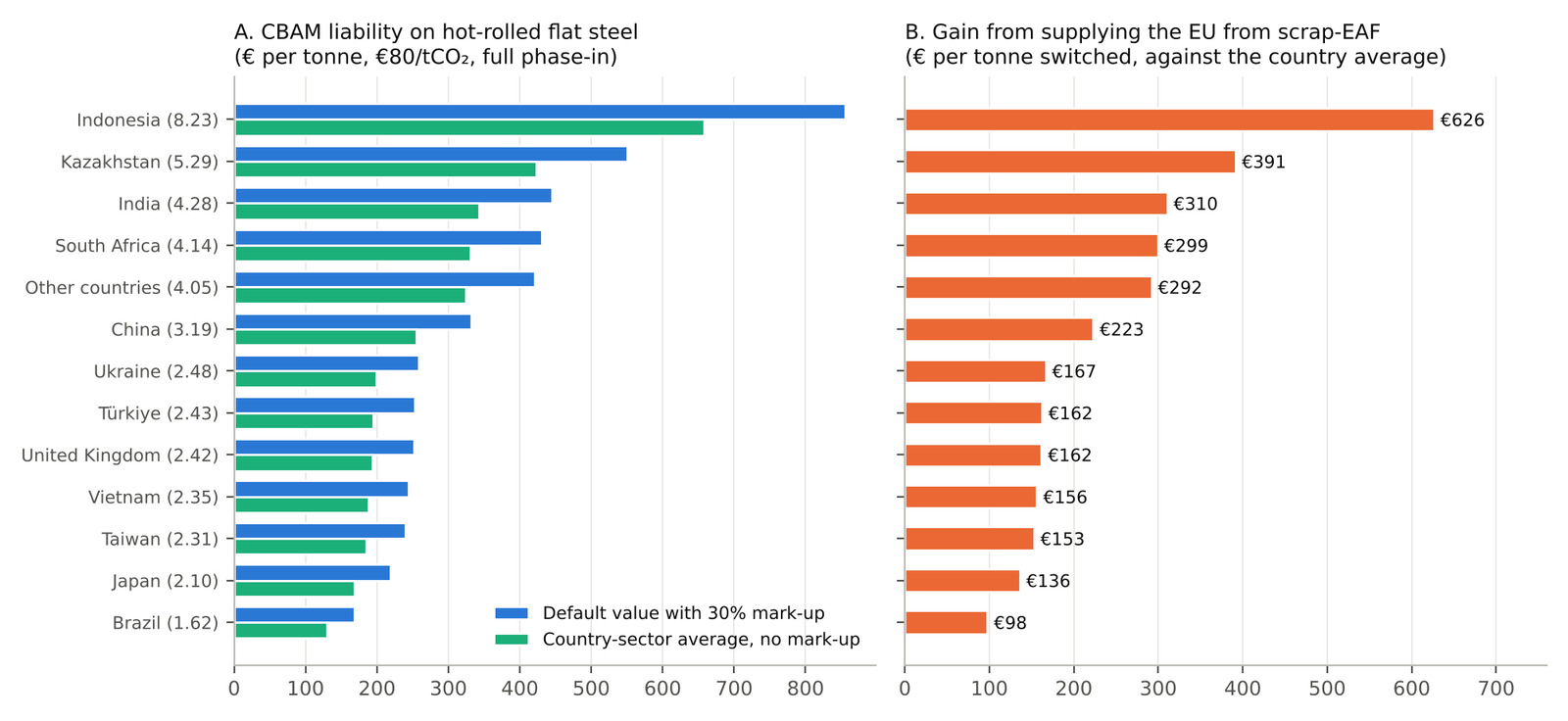
At €80 the liability on hot-rolled steel ranges from €168 to €856 per tonne under the marked-up defaults. Table 3 and panel A of Figure 2 show the liability under the default with mark-up and under the country-sector average without it. The mark-up alone is worth €39–198 per tonne. Indonesia’s default, 8.23 tCO₂/t, is an outlier that sets the top of the range; for the large exporters the liability is €445 for India, €331 for China and €252 for Türkiye.
2.Source/make_wp_figures.py.
| Exporter | Default value (tCO₂/t) | Liability, default with mark-up | Liability, country-sector average | Fall in liability on opting in, feebate at €40 | Fall in liability on opting in, feebate at €80 | Shuffling gain against the average | Shuffling gain against the marked-up default |
|---|---|---|---|---|---|---|---|
| Indonesia | 8.23 | 856 | 658 | 527 | 856 | 626 | 824 |
| Kazakhstan | 5.29 | 550 | 423 | 339 | 550 | 391 | 518 |
| India | 4.28 | 445 | 342 | 274 | 445 | 310 | 413 |
| South Africa | 4.14 | 431 | 331 | 265 | 431 | 299 | 399 |
| Other countries | 4.05 | 421 | 324 | 259 | 421 | 292 | 389 |
| China | 3.19 | 331 | 255 | 204 | 331 | 223 | 299 |
| Ukraine | 2.48 | 258 | 199 | 159 | 258 | 167 | 226 |
| Türkiye | 2.43 | 252 | 194 | 155 | 252 | 162 | 220 |
| United Kingdom | 2.42 | 252 | 194 | 155 | 252 | 162 | 220 |
| Vietnam | 2.35 | 244 | 188 | 150 | 244 | 156 | 212 |
| Taiwan | 2.31 | 240 | 185 | 148 | 240 | 153 | 208 |
| Japan | 2.10 | 218 | 168 | 134 | 218 | 136 | 186 |
| Brazil | 1.62 | 168 | 130 | 104 | 168 | 98 | 136 |
Opting in with a feebate is worth the whole liability at the EU price and about three fifths of it at half that price. A country that opts in with a feebate at €40 cuts the liability on its steel from the marked-up default to \((80 - 40)\bar e\): by €274 per tonne for India and €204 for China. Of India’s €274, €103 is the removal of the mark-up and €171 (\(40 \times 4.28\)) is recognition proper; for China it is €76 and €127 (rounded). The figures hold intensity at the default; the feebate itself would also cut intensity, by 24 percent at €40 in this calibration, and lower the liability further. At €80 the liability falls to zero: €445 and €331 per tonne. Under current rules the same feebate earns no recognition (Proposition 4), so the recognition part of these columns is the cost to exporters of the price-paid rule. For a country shipping 1 Mt of steel a year to the EU (a stylized volume), each €100 per tonne is €100 million a year.
2.Source/make_wp_figures.py.
Shuffling is worth €98–626 per tonne of steel routed: €160–310 million a year for each million tonnes that Türkiye, China or India can route. Panel B of Figure 2 gives the second form of equation 1 per tonne: the gain from supplying the EU with scrap-EAF steel rather than steel at the country average. For India it is €310 per tonne, for China €223 and for Türkiye €162. Against the marked-up default, which is the relevant comparison for an exporter that would otherwise not file data, the gains are €413, €299 and €220. The gain plateaus once scrap-EAF capacity covers EU sales (Proposition 1), so for a large exporter it is set by EU volumes, not by its scrap share. Sandbag’s scenario for China, at 2021 trade and full phase-in, is of the same order: fees on steel fall from €448 million to €259 million a year, and on all CBAM goods from €590 million to €313 million, when EU-bound steel is assumed to come from electric furnaces (Assous et al. 2024). None of these savings corresponds to lower emissions.
2.Source/make_wp_figures.py.
| Exporter | Default value (tCO₂/t) | Liability, default with mark-up | Liability, country-sector average | Gain from routing secondary metal |
|---|---|---|---|---|
| Mozambique | 3.20 | 333 | 256 | 227 |
| China | 3.00 | 312 | 240 | 211 |
| South Africa | 2.36 | 245 | 189 | 160 |
| Other countries | 2.20 | 229 | 176 | 147 |
| Russia | 2.16 | 225 | 173 | 144 |
| India, UAE, Bahrain | 1.87 | 194 | 150 | 121 |
| Brazil, Saudi Arabia | 1.70 | 177 | 136 | 107 |
For aluminum the gains are smaller per tonne but the same in kind. Routing remelted aluminum to the EU saves €107–227 per tonne against the country average (Table 4). The amounts are smaller than for steel only because CBAM counts direct emissions alone for aluminum.
Recognition raises the feebate rate an exporting country would choose for itself by a factor of 1.5 to 2.6. Figure 3 plots equation 3 and the adoption threshold. With a tenth of output sold to the EU, the country’s own best feebate rate is €8 under price-paid recognition and €21 with full recognition; at a quarter, €20 and €41; at a half, €40 and €62. A feebate at the full €80 pays for itself once more than half of output goes to the EU under the current rule, and once more than 24 percent goes there under full recognition. Neither threshold depends on the exporter’s intensity in this calibration, because the proportional abatement at a given rate is the same for all.
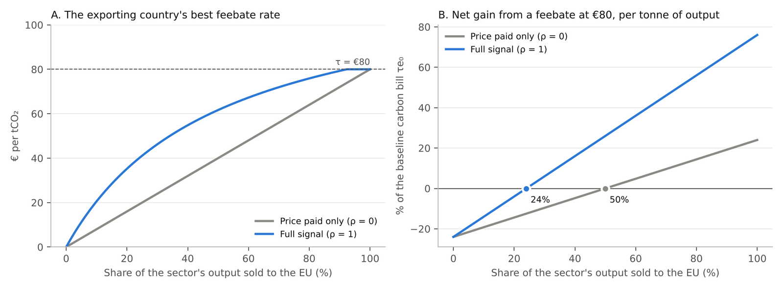
2.Source/make_wp_figures.py.
The calibration has three lessons. First, plant-level measurement puts at stake sums of the same order as the CBAM liability itself: for India the gain from routing a tonne is 91 percent of the country-sector liability on it. A rule that leaves this gain in place invites its capture, whatever the industrial frictions Mehling and Ritz (2023) rightly emphasize. Second, recognition is worth hundreds of euros per tonne to exactly the exporters with the highest intensities, who have the most to gain from adopting a feebate. Third, recognition alone does not make a feebate at the EU price attractive to a country selling a tenth of its steel to Europe. It moves the threshold from half to a quarter. Similar charges in other markets, which raise \(\mu\), and policy crediting (Stretton 2026e) would close the rest.
9 Legal pathway
Some of the design fits within the Commission’s existing powers; the central piece needs amendment. Four elements can be built by implementing act or through the default carbon price methodology.
Default carbon prices from 2027. Article 9(4) lets the Commission determine yearly default carbon prices for countries “where carbon pricing rules are in place”, using the best available data, and publish the methodology. An explicit feebate or rebated carbon tax is a carbon pricing rule. The methodology now being prepared for 2026–2028 starts from an inventory of emissions trading systems and carbon taxes (Technopolis Group 2026); the Commission could consult on it before adoption, base it on published measures (Agnolucci et al. 2024; Black et al. 2023; OECD 2023) and set it country by country and sector by sector.
Country-sector values without mark-up. The mark-up is set in the implementing acts under Article 7(7) “at an appropriate level to ensure the environmental integrity of the CBAM” (European Parliament and Council of the European Union 2025, Annex IV point 4.1). A country whose sector carries a recognized signal has supplied the incentive the mark-up exists to create, so setting its mark-up at zero is consistent with the stated purpose. Annex IV point 7 already admits region-specific adaptations of default values where declarants show, on reliable data, that they are lower. The revision of the default values due in 2027 (European Commission 2025f) is the natural vehicle, and its annual updating from verified data is what gives the country-sector value its incentive (Proposition 3).
The support test. Article 9(5) empowers the Commission to give “examples of any relevant rebate or other form of compensation”. The final implementing regulation can state the test of Section 6.2: output-based rebates are compensation for the price paid but not for the signal; abatement-contingent support meeting Article 8(2) is neither.
Shuffling. The Article 30 reports already cover resource shuffling (European Parliament and Council of the European Union 2023b, Art. 30). COM(2025) 989, still in co-decision, could add routing between installations under actual values to its circumvention clause (European Commission 2025g).
Recognizing the signal itself needs either a broad reading of “compensation” or an amendment. Article 9 credits a “carbon price … effectively paid” and requires “any rebate or other form of compensation … that would have resulted in a reduction of that carbon price” to be taken into account. A broad reading would hold that a rebate paid per unit of output does not reduce “the carbon price”, read as the rate per marginal tonne, and so is not compensation. The text resists it. Article 3(29) defines the carbon price as a “monetary amount paid”, an average, and the draft implementing regulation nets below-baseline emissions explicitly. Recognition of fuel excises and subsidy reform fails earlier still, because they are not levied on greenhouse gases as such and Article 9(4) admits defaults only where carbon pricing rules exist. The broad reading may carry the default carbon price for explicit feebates at the margin of the Commission’s discretion; the full design needs an amendment to Article 9 that adds the price signal, measured at country-sector level, as a ground for reduction. The 2027 revision of default values and the co-decision on COM(2025) 989 are the occasions.
Trade law favors recognizing comparable effort but scrutinizes treatment that differs by origin. Three provisions of the General Agreement on Tariffs and Trade (GATT) matter. Country-specific default values and default carbon prices treat like products differently by origin, which engages most-favored-nation treatment under Article I. If CBAM is characterized as an internal charge adjusted at the border, Article III:2 forbids taxing imports in excess of like domestic products, which bears on any measure, including a country-sector average, that charges a clean producer more than its actual intensity (Ismer and Neuhoff 2007; Mehling et al. 2019). The usual defense is the general exception for measures relating to the conservation of exhaustible natural resources or necessary to protect health, in Article XX(g) and (b), subject to the chapeau’s ban on “arbitrary or unjustifiable discrimination between countries where the same conditions prevail”. In US–Shrimp, the Appellate Body faulted a measure that required exporting countries to adopt essentially the same program as the United States, and later accepted one that required a program comparable in effectiveness (WTO Appellate Body 1998, 2001; Mehling et al. 2019). Recognizing the price signal, measured on a common scale for any instrument, is closer to the “comparable in effectiveness” standard than recognizing only explicit prices paid, and strengthens the chapeau defense. Two features of the design reduce the Article I and III risk: the criteria are origin-neutral, since any country that meets the signal threshold can opt in, and the verification route stays open to every exporter, so no producer is forced onto an average above its own verified intensity unless its government chose the country-sector route. Generous, rebuttable defaults reduce the risk further (Cosbey et al. 2019; Keen et al. 2022). A full legal opinion is beyond this paper.
10 Objections and limits
Recognition gives up part of the level playing field. This is the strongest objection. With full recognition, an exporter with a feebate at the EU price pays no CBAM charge on its average carbon, while EU producers pay on all their emissions once free allocation ends (Section 6.1). The relocation this invites, and its emissions consequence where the exporter remains dirtier than the EU producer, are not quantified here. The answer offered is to phase recognition in with the phase-out of free allocation, review relocation before each step, and price consumption separately (Stretton 2026e, 2026b).
The signal is harder to measure than the payment, and governments have reason to overstate it. Implicit prices and shadow prices of standards depend on modeled responses and elasticities (Stretton 2026d). Published measures, a phase-in and annual updating limit the risk; an independent body, such as a multilateral institution, could compute them.
No border measure resolves the exporter’s trilemma. An economy-wide carbon price raises costs on all output, competitiveness in markets without border adjustment needs low costs on output sold there, and trade rules forbid rebates contingent on export destination. One instrument can satisfy at most two. Signal recognition rewards a feebate that prices intensity without raising average costs, which eases the conflict, but the complete answer is two instruments: a production feebate and a destination-based consumption charge (Stretton 2026e, 2026b).
Country-sector averages pool clean and dirty plants. On the country-sector route a clean plant pays its country’s average. The recommended design accepts this only where the country chose it and its own signal rewards the clean plant. A country could also game the average, for instance by moving dirty capacity into a separately classified product. The default values’ CN-level detail limits this but does not remove it.
Shuffling across countries remains. Country-sector measurement removes routing within a country but not the movement of scrap between countries: a country can import scrap, lower its sector average and lower its CBAM bill while the exporting country of the scrap makes more ore-based steel (Proposition 2). Only a charge that values scrap at its opportunity cost, or global measurement of scrap flows, addresses this.
The model is partial equilibrium. It holds output, scrap supply and steel demand fixed or exogenous, and uses a quadratic abatement cost with stylized parameters. The shuffling and invariance results do not depend on these assumptions; the best-response rates and thresholds do.
Steel evidence is missing. No empirical study measures route shuffling in steel; the first study of trade under the definitive regime looks only at reallocation across countries and finds none yet (Hamidani 2026). The calibration gives the stakes, not the behavior. Installation-level CBAM declarations matched to customs data would allow the first measurement.
11 Conclusion and recommendations
CBAM measures embodied carbon plant by plant and credits only carbon prices paid. The first rule pays exporters €98–626 per tonne of steel to route scrap-based output to Europe with no change in emissions; the second gives nothing to a feebate that prices every tonne at the margin. Measuring embodied carbon by country and sector removes the first problem but leaves individual plants almost no incentive; crediting the country’s price signal restores it, and makes adopting a feebate worthwhile for an exporter that sells a quarter of its output to the EU rather than half. The main open question is empirical: how much routing between plants actually happens once installation-level declarations exist.
For the European Commission:
- Consult on the default carbon price methodology before it is adopted, build it on the World Bank, IMF and OECD measures, set it by country and sector, and let it cover feebates and non-price instruments measured as carbon-price equivalents.
- Adopt the two-route design of Section 7 in the 2027 revision of default values: verified country-sector values without mark-up, updated yearly, for sectors with a recognized price signal, and firm-level verification of whole output elsewhere.
- State the support test in the final implementing regulation on carbon prices paid: abatement-contingent support meeting Article 8(2) reduces neither the price paid nor the signal, output-based rebates reduce only the price paid, and emissions-contingent support reduces both.
- Propose an amendment to Article 9 that adds the country-sector price signal, measured as the switching-margin TECP, as a ground for reduction, with the recognition weight set each year to one minus the CBAM factor that governs free allocation (2.5 percent in 2026, about half in 2030, one from 2034 under current law, or later if the phase-out is extended), and a review of relocation before each step.
- Measure shuffling, using installation-level declarations matched to customs data, in the Article 30 reports, and extend the circumvention clause of COM(2025) 989 to routing between installations under actual values.
For exporting countries, a sector-wide feebate prices every tonne at a rate a tax could not reach politically, and is the instrument these changes would reward (Stretton 2026c).
Downloads
References
Appendix A: Literature review
This appendix adds detail to Section 4 by theme. Each entry in the bibliography records what was read: full text, abstract only, or the bibliographic record.
A.1 Border carbon adjustment design and recognition of foreign effort
The design literature treats recognition of foreign policy as one of a handful of core choices. Ismer and Neuhoff (2007) set out the early case that border adjustment for an emissions trading system can be made consistent with trade law if it is based on best available technology rather than actual foreign emissions. Cosbey et al. (2019), reviewing the literature for practitioners, list the regulatory choices: scope, the method for carbon content, the type and price of the adjustment, scenarios requiring modification, use of revenue, and compliance with trade and climate agreements. Mehling et al. (2019) give the most complete legal-economic analysis, tracing the Commission’s 2008 proposal that would have exempted partners taking “comparable action”; their analysis of the trade-law exceptions is the basis of Section 9. Kortum and Weisbach (2017) ask which goods, emissions and countries a border adjustment should cover, and conclude that adjustments impose high administrative costs and need stronger welfare justifications.
The two closest designs bracket this paper’s proposal. Mehling and Ritz (2023) propose a voluntary individual adjustment: a default intensity that a firm may rebut with its actual intensity, and a top-up charge on the shortfall of the foreign explicit carbon price, \(\max\{t - t_k, 0\} \times \min\{z, Z\}\). They do not include “effective” prices from non-price policies. Equation equation 2 with \(\rho = 0\) and plant-level \(\hat e\) is their rule; the paper’s generalization is to credit the signal and measure by country and sector. Neuhoff et al. (2026) go the other way: standardized values independent of process or location, free allocation at benchmark for EU producers, and a standardized liability per tonne of material, with export relief. That removes shuffling and keeps carbon-pricing incentives along the EU value chain, but by their own account creates no direct incentive for cleaner production or carbon pricing abroad. The country-sector route of Section 7 sits between the two: no plant can shuffle, and the exporting country is rewarded for its own instrument.
Recent work recommends starting simple and moving to finer measurement. Keen et al. (2022) judge border adjustments the most effective unilateral instrument against competitiveness loss and leakage, but stress that design is decisive. They recommend limiting coverage to energy-intensive, trade-exposed sectors, benchmarking initially on domestic emission intensities, and deciding explicitly how to treat partners that mitigate by other means. They show that output-based rebating of a carbon tax is a feebate, the equivalence this paper uses. Clausing and Wolfram (2023) separate free-riding by low-ambition countries from the competitive disadvantage of jurisdictions that price carbon against those that subsidize clean production, and show that one border instrument cannot address both. A feebate, which prices at the margin and subsidizes on average, sits between their two cases, which is why price-paid recognition misjudges it.
Leakage estimates bound what is at stake. Branger and Quirion (2014)’s meta-analysis of 25 studies and 310 estimates finds leakage rates of 5–25 percent without border adjustment (mean 14 percent) and 5–15 percent with it (mean 6 percent); extending the adjustment to all sectors is the most effective feature. Fischer and Fox (2012) compare border adjustment with output-based rebating as anti-leakage tools.
A.2 Who bears CBAM
Exposure falls disproportionately on middle- and low-income exporters with weak verification capacity. Beaufils et al. (2023) find that middle- and low-income countries for which the EU is an important market are hit hardest relative to their economies, even under conservative designs, and explore international schemes for recycling the revenue. Magacho et al. (2024) find Russia, China, Türkiye and Ukraine most exposed in absolute terms, many developing economies with more than 2 percent of exports and 1 percent of production affected, and the Western Balkans, Mozambique, Zimbabwe and Cameroon most exposed relative to their economies. Eicke et al. (2021) build a risk index that includes capacity for monitoring, reporting and verification, and find most high-risk countries in Africa. Perdana and Vielle (2022) find in a general equilibrium model that CBAM cuts leakage by about a third by 2040 but reduces welfare in the least developed countries through lower exports; exempting them raises leakage more than alternatives, while returning revenue for clean energy improves their welfare at low cost to the EU. Mattoo et al. (2009) show, for border taxes set on each exporter’s carbon content, that the burden falls heavily on poorer exporters: China’s manufacturing exports fall by about a fifth, and those of low- and middle-income countries by about 8 percent. These findings matter for recognition because the countries most exposed are those least able to file verified plant data, for which the default values and default carbon prices are the only routes.
A.3 Resource shuffling and leakage under incomplete regulation
The quantitative evidence on shuffling comes from electricity. Fowlie (2009) simulates California’s electricity market under source-based cap-and-trade and finds that exempting out-of-state producers achieves about a third of the reductions of complete regulation at more than twice the cost per tonne. Caron et al. (2015) find that California’s program without restrictions on imported electricity would raise emissions elsewhere by 45 percent of its domestic reduction; with imports in the cap and resource shuffling banned as legislated, leakage falls to 9 percent. The 9 percent assumes the ban works, and Mehling and Ritz (2023) report that it has been difficult to enforce. Fowlie and Reguant (2022) show how to calibrate output subsidies to leakage risk in incomplete carbon markets, which bears on how free-allocation benchmarks should be set. Apaydın (2026) shows the same gap between reported and real cuts in a new place: under CBAM’s electricity-accounting rules, Chinese industrial parks can report reductions of which only about a fifth to a quarter are real in some provinces.
The leading analysis of industrial goods expects less shuffling than in electricity, but offers no measurement. Mehling and Ritz (2023) judge reshuffling “perhaps most acute for electricity markets” and likely less pronounced for industrial goods, whose flows are easier to trace, and suggest a company-level point of regulation. This paper’s Proposition 6 formalizes their trade-off, and the firm-level verification route in Section 7 is their remedy. Their expectation of smaller industrial shuffling is plausible for routing that requires changing physical flows. It is weaker for routing between installations owned by one firm, which requires only that the firm choose which plant fills which order, and for selection into country-average default values, which requires nothing at all.
For steel there are scenario estimates and no measurement of routing. Assous et al. (2024) estimate CBAM fees on imports from China at 2021 trade volumes and full phase-in: €590 million with unchanged flows, €313 million if exporters supply the EU only with electric-furnace steel (half scrap and half direct-reduced or pig iron for flat products), aluminum made with 80 percent scrap and cement with 20 percent clinker, and €695 million with no reporting. They note that the Commission must monitor resource shuffling under Article 30 but has no enforcement mechanism. Hamidani (2026) tests, with monthly customs data for 52 flat-steel products in January–June 2026, whether origins with higher default-based exposure lost EU business, and finds no stable effect yet. A Crossref search on 31 October 2026 found no empirical paper on routing between scrap-EAF and BF-BOF output to the EU.
A.4 Measuring carbon prices beyond explicit ones
Implicit carbon pricing through fuel taxes and subsidies is most of the world’s carbon price, and measures of it exist. Agnolucci et al. (2024) develop a total carbon price that adds indirect pricing, fuel excise taxes net of subsidies, to explicit carbon taxes and emissions trading, for 142 countries from 1991 to 2021. Direct pricing covers roughly a quarter of global emissions, but the global total carbon price is not much higher than in 1994, and indirect pricing still makes up “the lion’s share”. Many developing countries, especially net fuel importers, contribute substantially once indirect pricing counts. Black et al. (2023) estimate efficient fuel prices that reflect supply and environmental costs, and the subsidies implied by charging less. The OECD’s effective carbon rates add carbon taxes, fuel excise taxes and permit prices by country and sector (OECD 2023). All three measure the average price per tonne. Paper 6.1 converts any instrument, including feebates and standards, into the uniform tax that would cut emissions as much, and separates the fuel-switching margin from the demand margin (Stretton 2026d); its switching-margin price is the price signal in equation 2.
A.5 Intensity-based pricing and refunding
Instruments that price intensity and return revenue by output are well understood, and are exactly what price-paid recognition misses. Output-based allocation, tradable performance standards and feebates charge the full rate on emissions at the margin while returning revenue in proportion to output, so they subsidize output relative to a tax (Fischer 2001; Fischer and Fox 2012). Holland et al. (2009) show that an intensity standard can even raise emissions when its implicit output subsidy is large. Paper 1.2 of this series designs feebates for power and industry (Stretton 2026c). Hagem et al. (2020) compare refunding emission payments by output with refunding in proportion to abatement spending: expenditure-based refunding needs a lower fee than a tax for the same abatement, output-based refunding a higher one, and both tilt effort toward abatement technology rather than output. This is the economic content of the draft implementing regulation’s Article 8(2) exemption for revenue-financed decarbonization support, and the basis of the support test in Section 6.2.
A.6 Trade law and comparable effort
The trade-law literature favors recognizing foreign effort and warns against treating like products differently by origin. Ismer and Neuhoff (2007) argue that a border adjustment levied as an internal charge can be defended under the GATT if it charges imports no more than domestic producers would pay with the best available technology. Mehling et al. (2019) analyze the full chain: whether a carbon border charge is an internal tax adjustable at the border, whether products differing only in how they were made are “like”, and the general exceptions of Article XX, whose chapeau forbids “arbitrary or unjustifiable discrimination between countries where the same conditions prevail”. The US–Shrimp disputes are the main precedent: the Appellate Body faulted an import ban that in effect required exporting countries to adopt the same program as the United States, and later accepted a revised measure that required a program comparable in effectiveness (WTO Appellate Body 1998, 2001). For recognition, a test of comparable effect, applied by criteria any country can meet, is safer than one that credits only instruments resembling the importer’s own.
Country-level measures raise their own trade-law questions. Country-specific default values and default carbon prices treat like products differently by origin, which engages most-favored-nation treatment under Article I. Cosbey et al. (2019) and Keen et al. (2022) recommend generous defaults that individual producers can rebut with their own data. The country-sector route of Section 7 departs from this by removing the individual rebuttal for countries that opt in; its defense is that the exporting government chooses it, that the criteria are origin-neutral, and that the verification route stays open to every other exporter. Whether that defense would hold has not been tested.
A.7 What this paper adds
Four points stand against the literature and the legal texts. First, the default carbon price is the operative recognition route for most exporters, and the law makes it discretionary, from 2027, and confines it to countries with carbon pricing rules; for countries with only implicit pricing it is zero by construction. Second, the draft implementing regulation’s Article 8(1)(b)(ii) nets below-baseline emissions, so a feebate or output-based pricing system is recognized only on emissions above its benchmark, although its marginal signal is the full rate; Proposition 4 formalizes this. Third, plant-level measurement creates two routes to shuffling, routing under actual values and selection into country-average default values, neither of which the Commission’s anti-circumvention proposal addresses, while country-sector measurement removes both but leaves plants almost no incentive (Propositions 1–3 and 6). Fourth, a liability formula that credits the country-sector price signal is invariant to shuffling, restores the plant incentive through the exporter’s own instrument and preserves the best-response property of paper 1.1, at a cost to the level playing field that Section 6.1 makes explicit.
Appendix B: Proofs
Proposition 1. The plant-level bill \(B(x) = \tau[e_S x + e_B(Q_{EU} - x)]\) has \(B'(x) = -\tau(e_B - e_S) < 0\). With routing cost \(c\) per tonne moved, the net gain from moving a tonne is \(\tau(e_B - e_S) - c > 0\), so the exporter sets \(x\) at its upper bound \(\min(q_S, Q_{EU})\). The saving relative to \(x_0 = sQ_{EU}\) is \(B(x_0) - B(x^*) = \tau(e_B - e_S)[\min(q_S, Q_{EU}) - sQ_{EU}]\), gross of routing costs. If \(q_S \ge Q_{EU}\) this is \(\tau(e_B - e_S)(1-s)Q_{EU}\); substituting \(e_B = (\bar e - s e_S)/(1-s)\) gives \(\tau(\bar e - e_S)Q_{EU}\). If \(q_S < Q_{EU}\) it is \(\tau(e_B - e_S)\,s\,(Q - Q_{EU})\). Total emissions \(e_B q_B + e_S q_S\) do not depend on \(x\). When \(q_S \ge Q_{EU}\), \(x^* = Q_{EU}\) and \(B = \tau e_S Q_{EU}\), so \(\partial B/\partial e_B = 0\). In the stylized example, \(\tau(e_B - e_S)(1-s)Q_{EU} = 80 \times 1.6 \times 0.8 \times 1 = 102.4\) (€ million).
Proposition 2. Reported embodied carbon in EU imports falls by \((e_B - e_S)\Delta\) because \(\Delta\) tonnes previously supplied at \(e_B\) are now supplied at \(e_S\). Globally, the exporter’s emissions fall by \((e_B - e_S)\Delta\) if the new scrap-EAF output replaces its own BF-BOF output. Of the \(\Delta\) tonnes of scrap used, \(\theta\Delta\) are newly collected and \((1-\theta)\Delta\) are diverted from other users, who replace their scrap-based output at intensity \(e_R\), raising their emissions by \((e_R - e_S)(1-\theta)\Delta\). The net change is \(-(e_B - e_S)\Delta + (1-\theta)(e_R - e_S)\Delta\), equal to \(-\theta(e_B - e_S)\Delta\) when \(e_R = e_B\) and zero when also \(\theta = 0\). Pure rerouting leaves every plant’s output unchanged, so world emissions are unchanged for any \(\theta\).
Proposition 3. (i) \(B_C = \tau\bar e Q_{EU}\) with \(\bar e = \sum_i q_i e_i / Q\) contains no routing variable; every plant is charged at \(\bar e\), so the choice between actual and default values does not arise. (ii) \(\partial B_C/\partial e_i = \tau Q_{EU} q_i/Q = \tau\mu q_i\), which is \(\tau\mu\) per tonne of plant \(i\)’s output. (iii) Firm \(f\)’s own bill is \(\tau\bar e\,Q_{EU,f}\) with \(Q_{EU,f} = \mu_f q_f\), so \(\partial(\tau\bar e\,Q_{EU,f})/\partial e_f = \tau\mu_f q_f \cdot q_f/Q\), which is \(\tau\mu_f\sigma_f\) per tonne of firm \(f\)’s output with \(\sigma_f = q_f/Q\). (iv) If the value charged is fixed for a period, the bill does not depend on any \(e_i\) within it.
Proposition 4. (i) \(\sum_i q_i t(e_i - \bar e) = t(\sum_i q_i e_i - \bar e\sum_i q_i) = 0\) with \(\bar e = \sum_i q_i e_i/\sum_i q_i\). (ii) A plant with \(e_i > \bar e\) pays \(t(e_i - \bar e)\) per tonne of output; a plant with \(e_i \le \bar e\) receives a rebate, which under netting of below-baseline emissions leaves a recognized price paid of zero (the reduction cannot be negative). (iii) The scrap-route plant has \(e_S < \bar e\), so its recognized deduction is zero and its EU bill is \(\tau e_S\); a BF-BOF tonne’s bill is \(\tau e_B - t(e_B - \bar e)\), which with \(t = \tau\) is \(\tau\bar e\), so routing saves \(\tau(\bar e - e_S)\). (iv) A tax at rate \(t\) is paid in full, \(t e_i\) per tonne of output, and induces \(e_i = e_{0i} - t/k_i\), the same intensity as a feebate at \(t\) (Stretton 2026e, Prop. 2).
Proposition 5. (i) \(\bar e_{c,s}\), \(p_{c,s}\) and \(t^{\mathrm{sig}}_{c,s}\) are sector aggregates. (ii) For \(\rho t \le \tau\), \(D(t) = c_0 + t^2/2k + (\tau - \rho t)(e_0 - t/k)\), so \(D'(t) = [(1+2\rho)t - \tau]/k - \rho e_0\) and \(D''(t) = (1+2\rho)/k > 0\). The stationary point is \(t = (\tau + \rho k e_0)/(1 + 2\rho)\). At \(\rho = 0\) it is \(\tau\). At \(\rho = 1\) it is \((\tau + k e_0)/3\), which exceeds \(\tau\) by \((k e_0 - 2\tau)/3 \ge 0\) when \(k e_0 \ge 2\tau\); then \(D\) is decreasing on \([0, \tau]\), and for \(t > \tau\) the liability is zero and \(D = c_0 + t^2/2k\) is increasing, so the minimum is at \(t = \tau\). \(D_{\rho=0}(\tau) - D_{\rho=1}(\tau) = \tau(e_0 - \tau/k)\). For \(0 < \rho < 1\) the minimizer is \(\min\{(\tau + \rho k e_0)/(1 + 2\rho), \tau/\rho\}\), which is at least \(\tau\) when \(k e_0 \ge 2\tau\). (iii) Per unit of output the country’s net cost is \(N(t) = t^2/2k + \mu(\tau - \rho t)(e_0 - t/k)\); \(N'(t) = t/k - \mu[\rho e_0 + \tau/k - 2\rho t/k] = 0\) gives equation 3, \(N''(t) = (1 + 2\rho\mu)/k > 0\), and \(\partial t^*/\partial\rho = \mu(k e_0 - 2\mu\tau)/(1 + 2\rho\mu)^2\). (iv) At \(\rho = 0\) the CBAM saving from \(t = \tau\) is \(\mu\tau\cdot\tau/k\) against a resource cost \(\tau^2/2k\), so the net gain is \((\tau^2/k)(\mu - 1/2)\). At \(\rho = 1\) the saving is the whole liability \(\mu\tau e_0\), so the net gain \(\mu\tau e_0 - \tau^2/2k\) is positive if and only if \(\mu > \tau/(2k e_0)\). The implied price per tonne abated of the relief is \(\mu\rho t\bar e/(t/k) = \mu\rho k\bar e\).
Proposition 6. The bill on a tonne from unit \(i\) is \(\tau[\lambda e_i + (1-\lambda)\bar e_{c,s}]\), so \(\partial(\cdot)/\partial e_i = \lambda\tau\) (ignoring unit \(i\)’s own small weight in \(\bar e_{c,s}\)), and the difference between supplying from \(B\) and from \(S\) is \(\lambda\tau(e_B - e_S)\).
All results were checked symbolically (2.Source/check_propositions.py).
Appendix C: Legal texts and status
The list comes from the EU Publications Office, from which the main texts were read on 31 October 2026, and from the Commission’s Have Your Say portal (initiative 14830), queried the same day.
| Act | Subject | Adopted | Official Journal | Status at 31 October 2026 |
|---|---|---|---|---|
| Regulation (EU) 2023/956 (European Parliament and Council of the European Union 2023b) | Establishes CBAM | 10 May 2023 | L 130, 16.5.2023, p. 52 | In force; definitive period from 1 January 2026; Article 9 replaced by 2025/2083 |
| Directive (EU) 2023/959 (European Parliament and Council of the European Union 2023a) | EU ETS revision; CBAM factor phasing out free allocation 2026–2034 | 10 May 2023 | L 130, 16.5.2023, p. 134 | In force |
| Implementing Regulation (EU) 2023/1773 (European Commission 2023) | Reporting in the transitional period | 17 August 2023 | L 228, 15.9.2023, p. 94 | Transitional period ended 31 December 2025 |
| Regulation (EU) 2025/2083 (European Parliament and Council of the European Union 2025) | Simplification: 50-tonne threshold; new Article 9; default values at country averages plus mark-up; certificate sales from 1 February 2027 | 8 October 2025 | L, 2025/2083, 17.10.2025 | In force |
| Delegated Regulation (EU) 2025/2551 (European Commission 2025a) | Accreditation of verifiers | 20 November 2025 | L, 2025/2551, 22.12.2025 | In force |
| Implementing Regulation (EU) 2025/2546 (European Commission 2025b) | Verification principles | 10 December 2025 | L, 2025/2546, 22.12.2025 | In force |
| Implementing Regulation (EU) 2025/2547 (European Commission 2025c) | Methods for calculating embedded emissions | 10 December 2025 | L, 2025/2547, 22.12.2025 | In force |
| Implementing Regulation (EU) 2025/2548 (European Commission 2025d) | Price of CBAM certificates | 10 December 2025 | L, 2025/2548, 22.12.2025 | In force |
| Implementing Regulation (EU) 2025/2620 (European Commission 2025e) | Free-allocation adjustment; benchmarks by production route | 16 December 2025 | L, 2025/2620, 22.12.2025 | In force |
| Implementing Regulation (EU) 2025/2621 (European Commission 2025f) | Default values by country, with mark-ups of 10, 20 and 30 percent (1 percent for fertilizers) | 16 December 2025 | L, 2025/2621, 31.12.2025 | Applies from 1 January 2026; to be revised in 2027 at the latest |
| COM(2025) 783 (European Commission 2025h) | Report on the application of CBAM | 16 December 2025 | not in OJ | Published |
| COM(2025) 989, 2025/0419(COD) (European Commission 2025g) | Downstream goods; anti-circumvention, including supply chains adjusted to reach lower default values; pre-consumer scrap as precursor | 17 December 2025 | not in OJ | Pending in co-decision |
| Draft implementing regulation, Ares(2026)4841230 (European Commission 2026a) | Carbon price paid in a third country: conversion, evidence, independent persons | Draft of 13 May 2026 | not in OJ | 177 feedback responses; in adoption workflow; not adopted |
| COM(2026) 616, 2026/0212(COD) (European Commission 2026b) | EU ETS amendment: free allocation to CBAM sectors phased out by 2038 | 17 July 2026 | not in OJ | Under negotiation |
Provisions quoted in the paper. Regulation 2023/956, Article 3(29): definition of carbon price; Article 30: reports on “international trade, including resource shuffling”; Annex II: direct emissions only for iron and steel and aluminum. Article 9(1)–(5) as replaced by Regulation 2025/2083: deduction for carbon price effectively paid, available where actual emissions are declared; netting of “any rebate or other form of compensation”; yearly default carbon prices “only where a carbon price was set by the rules applicable in the third country and a yearly default carbon price can be determined, including on a conservative basis”; the Commission “may” determine default carbon prices from 2027 “for third countries where carbon pricing rules are in place” and publish the methodology; implementing acts on conversion, evidence and examples of compensation. Regulation 2025/2083, recital 20 (annual average price “including on a conservative basis”) and recital 35 (ten-highest-intensity rule); Annex IV, point 4.1 (default values at country averages plus a mark-up set under Article 7(7)) and point 7 (region-specific adaptations). Directive 2023/959: CBAM factor 97.5 percent in 2026, 95 in 2027, 90 in 2028, 77.5 in 2029, 51.5 in 2030, 39 in 2031, 26.5 in 2032, 14 in 2033, none from 2034. Draft implementing regulation: recital 8 (binding mechanisms imposing obligations on all operators), Article 6 (conversion formulas), Article 8(1)(b)(ii) (below-baseline emissions as compensation), Article 8(2) (revenue-financed subsidies not netted under four conditions), and the 10 percent cap on Paris Agreement Article 6 credits.
Appendix D: Calibration data and code
Data. The default values are the Commission’s, as adopted under Implementing Regulation (EU) 2025/2621 (European Commission 2025f); only the values in the Regulation are legally valid. For each of 119 countries and a residual “other countries” category, and for each CN code, the Regulation gives the direct, indirect and total default values, the values with the 2026, 2027 and 2028-onward mark-ups, and the production-route code that determines the CBAM benchmark. For steel and aluminum the indirect values are not applicable. The calibration uses direct values before mark-up for hot-rolled flat steel (CN 7208) and unwrought aluminum (CN 7601), extracted to ../1.1.OpenEconomyCarbonPricing/2.Source/CBAM-default-values-steel-aluminium-cement.csv and checked on 31 October 2026 against the Official Journal text for every country in Table 3 and Table 4. Every steel exporter in Table 3 carries route code (C), carbon steel by BF/BOF; unwrought aluminum carries (K), primary aluminum, or (L), secondary aluminum at 0.36 tCO₂/t, as the Regulation’s legend defines them. No World Bank internal data are used.
Stylized parameters. Certificate price €80/tCO₂. Full phase-in, with no free-allocation adjustment. Mark-up 30 percent. Scrap-EAF steel 0.4 tCO₂/t and BF-BOF steel 2.0 tCO₂/t in the worked example, against the IEA’s 0.3 and 2.2 (direct plus indirect) and 0.04 and 1.2 (direct) (International Energy Agency 2020). Secondary aluminum 0.36 tCO₂/t. Abatement cost \(c(e) = c_0 + \tfrac{k}{2}(e_0 - e)^2\) with \(k = 50/(0.3\,e_0)\), so that a rate of 50 cuts intensity by 30 percent and \(k e_0 = €166.7\)/tCO₂ for every exporter, as in paper 1.1 (Stretton 2026e). At €80 the induced intensity cut is 48 percent, so the condition \(k e_0 \ge 2\tau\) of Proposition 5(ii) holds.
Code. 2.Source/make_wp_figures.py reads the data, writes table_steel.csv and table_aluminium.csv (the source of Table 3 and Table 4) and draws Figure 1, Figure 2 and Figure 3. 2.Source/check_propositions.py checks Propositions 1–6 symbolically with SymPy and reproduces the numbers quoted from them: the €102 million saving in the worked example, the best-response rates of €8 and €21 at \(\mu = 0.1\), the 24 percent adoption threshold, and the €0.80 private incentive in the example of Proposition 3.