Public Investment in CPAT
Investment Needs and the Efficiency of Public Spending
Carbon pricing models tell a finance ministry what a policy raises and what it cuts, but not what the clean capital it calls for will cost or whether the budget should pay for it. This paper extends the Climate Policy Assessment Tool in two directions. The first turns physical change into investment needs by country and sector and prices that capital at three rates: the market cost of capital, a social rate, and a social rate with co-benefits counted. For a stylized asset whose fuel savings are 13.3 cents a year per dollar of capital, the financial case fails above a cost of capital of 12.6 percent, the rate the tool’s optional income-group setting gives lower-middle-income countries. The second extension asks what each dollar of net public money buys, against the cost of raising tax, with haircuts for delivery and with capital, operating and contract routes on one fiscal ledger. In a stylized island case a solar plant worth $108 million passes that test on every route, but a seven-year loan leaves the budget $14.6 million a year short; concessional finance closes the gap, and a guaranteed power purchase agreement narrows it by turning debt into a contract liability. Country runs put 2030 investment needs in Kenya, Uganda and St Lucia at 4 to 5 percent of GDP, and a run of the open SISEPUEDE model for Uganda shows that under a fifth of its net-zero benefits reach the budget as cash.
investment needs, cost of capital, marginal cost of public funds, marginal value of public funds, public investment efficiency, power purchase agreements
Working paper, version 0.2, October 2026. Stephen J. Stretton, writing in a personal capacity. The views expressed are the author’s own and do not represent those of any institution with which he is or has been affiliated. A short version for policy makers is Climate Fiscal Policy Brief No. 6.3. Companion paper to the public CPAT-AI repository, https://github.com/cpmodelai/cpat_ai.1
1 Executive summary
Policy brief (short version) → · Download this paper (pdf) · Slides (pdf)
A finance ministry that prices carbon also needs to price the clean capital the policy calls for. The Climate Policy Assessment Tool (CPAT), built by the World Bank and the International Monetary Fund (IMF), tells a ministry what a carbon tax raises and what it cuts in more than 180 countries. It does not say what the wind farms, grids and electric buses the policy calls for will cost to finance, who should pay, or whether public money spent on them beats money left with taxpayers. Developing countries other than China need $2.3 to 2.5 trillion a year of climate investment by 2030.
This paper adds two extensions to CPAT. The first turns the physical change CPAT already computes into investment needs by country and sector and prices that capital three ways: at the market cost of capital each country faces, at the World Bank’s 6 percent social rate, and at 6 percent with co-benefits such as cleaner air counted. The second scores each use of public money by what people get per dollar the budget really pays, and funds it when that ratio beats the cost of raising a dollar of tax, about 1.2 in African evidence.
The cost of capital, not the size of the bill, decides whether clean capital pays its way. A stylized asset that saves 13.3 cents a year in fuel and running costs per dollar of capital, over 25 years, pays its way only if it is financed below 12.6 percent. That is the rate CPAT’s optional income-group setting assigns to lower-middle-income countries (12.5 percent). CPAT’s default setting instead adds a technology premium of about 3 points for wind and solar to each country’s own cost of capital, so a lower-middle-income country’s solar asset crosses the line once its country rate passes about 9.7 percent. Applied at the scale of the expert group’s 2030 estimates, the same capital that earns developing countries $131 billion a year at 6 percent earns them only $45 billion at a 10.5 percent market rate.
The gap between what investors see and what society gets is the case for public finance. Pricing carbon and air pollution, concessional lending, and guarantees or pooling that cut the risk premium all close it. Each point off the cost of capital is worth about $36 billion a year for each year’s clean energy investment of $4.8 trillion.
The budget’s problem is often cash and debt statistics, not value. In a stylized small island with 85 percent public debt, a $120 million solar plant that replaces diesel is worth $108 million at 6 percent and passes the public-money test on every financing route. But the only commercial loan, at 8 percent over seven years, leaves the budget $14.6 million a year short for seven years and adds 6 percent of GDP to headline debt. A concessional loan puts cash into the budget from the first year. A power purchase agreement keeps the debt off the books but commits the island to payments worth 7.6 to 8.9 percent of GDP, more than the debt it avoids. A constant cost of public funds cannot see this trap.
Country runs show the same pattern on real data. The investment-needs tool puts 2030 mitigation investment at 4.7 percent of GDP in Kenya, 4.0 percent in Uganda and 4.4 percent in St Lucia. In Kenya and Uganda the incremental investment is a net cost at market rates and at 6 percent and pays only when cleaner air is counted; in St Lucia, which burns imported diesel, it pays at any rate. A SISEPUEDE run for Uganda values its net-zero strategy at $161 billion at 6 percent, but only 18 percent of the benefits are cash a budget or utility would see.
What to do. Teams running CPAT should report investment needs at the country’s own cost of capital and at 6 percent side by side, and say which cost-of-capital setting they used. Ministries should test public measures against a cost of public funds that rises in cash-short years, and count a power purchase agreement’s committed payments as a liability. The CPAT team should publish a table of the cost of capital by country and technology. The policy brief sets out what this means for finance ministries.
2 Introduction
Developing countries other than China need about $2.3 to 2.5 trillion a year of climate investment by 2030, out of a world total of $6.3 to 6.7 trillion (Bhattacharya et al. 2024). The headline hides two questions a finance minister must answer before any of it is built. The first is what the capital costs to carry. For a solar plant, money is most of the price: the International Energy Agency finds that the cost of capital for utility-scale solar in emerging and developing economies is well over twice that in advanced economies (International Energy Agency 2024), and the same plant financed at 12 percent rather than 4 percent sells power for about 80 percent more (Stretton 2026c). The second is whether the budget should pay at all, and if so how. A plant that pays back handsomely in economic terms can still break a budget that must service a seven-year loan, and a power purchase agreement that keeps the plant off the debt statistics can cost more than the debt it avoids.
The Climate Policy Assessment Tool (CPAT) answers neither question. CPAT, built by the International Monetary Fund (IMF) and the World Bank, projects fuel use, emissions, revenue and welfare for more than 180 countries under carbon taxes, subsidy reform and related policies (Black et al. 2023; CPAT Team 2024). Its power model chooses new capacity on levelized cost at a cost of capital set by country and technology, and reports investment spending by technology. But outside power it has no capital at all, it does not split investment between public and private payers, and it has no test of whether a dollar of public spending on clean capital beats a dollar left with taxpayers. Its revenue side is rich; its spending side is a list of uses of revenue.
This paper asks how CPAT can be extended to estimate climate investment needs, price them at the cost of capital countries actually face, and test whether public money should pay for them. The answer has two parts. The first extension (investment needs) multiplies physical change by unit capital cost, turns capital into an annual charge with a capital recovery factor, and reports the result through three lenses: the market cost of capital, the World Bank’s 6 percent social rate, and the social rate with co-benefits and carbon counted. The gap between the first and third lens is the case for public finance and de-risking. The second extension (spending efficiency) scores each candidate use of public money by the ratio of what people get to what the budget really pays, after removing what the private sector would have done anyway, money that never becomes a working asset, and money that comes back. A measure is funded if that ratio exceeds the marginal cost of public funds, about 1.2 in African evidence (Auriol and Warlters 2012). With a cost of public funds of 1 and no budget limit, the rule reduces to the World Bank’s usual net present value test.
Four results follow. A stylized asset with fuel savings of 13.3 cents a year per dollar of capital and a 25-year life has a financial case only below a cost of capital of 12.6 percent (Proposition 1), which is where CPAT’s optional income-group rate for lower-middle-income countries sits. The spending test nests World Bank practice and prices revenue returns at the cost of public funds (Proposition 2). Stretching loan tenor eases liquidity but does not change solvency, so a single cost of public funds cannot see a cash trap (Proposition 3). A power purchase agreement priced at a cost of capital above the government’s borrowing rate is debt in disguise, and without mid-life replacements its committed payments are worth more than the plant (Proposition 4). A worked example for a stylized small island shows all four at once, and country runs for Kenya, Uganda and St Lucia apply the lenses to tool results.
The paper adds to three strands of work, and its contribution is to join them inside a model ministries already use. Investment-needs studies differ mainly in what they count and at what rate (Rozenberg and Fay 2019; Bhattacharya et al. 2024; Kalra et al. 2023); this paper puts the cost of capital by country and technology inside the estimate and reports the three lenses side by side. Integrated-model studies show the cost-of-capital premium and its effect on decarbonization (Steffen 2020; Ameli et al. 2021; Calcaterra et al. 2024) but stop before the budget. The marginal value of public funds (Hendren and Sprung-Keyser 2020; Finkelstein and Hendren 2020) has been applied mostly to United States social policy; this paper applies it to climate capital in low-capacity states, with delivery haircuts from the public investment efficiency literature (Pritchett 2000; International Monetary Fund 2015) and with financing routes and contract liabilities on one ledger. The propositions are short, and two of them restate known facts in this setting; their use is that they put numbers on those facts inside a ministry’s model.
3 What CPAT computes and what it lacks
CPAT already computes most of the physical change an investment estimate needs, but only in power does it attach capital to it. CPAT projects each fuel in each sector from last year’s use, output and prices; paper 5.1 states the method (Stretton 2026f). Its power model retires plants, dispatches the rest and builds new capacity, sharing new investment among technologies with a logit function of levelized cost and capping how fast wind and solar can grow (CPAT Team 2024). So CPAT knows how many megawatts a carbon price adds, at what rate they are financed and what they cost, and its power model reports investment spending by technology. Outside power it has no capital at all: an efficiency gain in industry or a shift to electric cars appears as lower fuel use, not as an investment someone must make.
CPAT’s default cost of capital is a country rate plus a technology premium; rates by income group are an option. The 2023 documentation describes the cost of capital as “by default income-dependent”: 7.5 percent in high-income, 10 percent in upper-middle-income, 12.5 percent in lower-middle-income and 15 percent in low-income countries, following Steffen (2020; CPAT Team 2024). The model’s own setting, which the rebuilt CPAT-AI workbook follows, is different. It takes each country’s real cost of capital for 2022 from a calculator built on a real risk-free rate, country risk premiums and default spreads (7.5 percent where a country is missing), and adds a technology premium that depends on income group: in lower-middle-income countries about 2.5 points for coal, gas and oil plants and 2.9 points for wind and solar (CPAT-AI Project 2026). The income-group rates are used only when the user selects them. Paper 5.1 records the same difference (Stretton 2026f). The default is closer to what this paper needs, because it varies by country and technology; but its country table is not published as data, and the premium is a judgment, not an estimate.
CPAT’s fiscal accounts stop at revenue. CPAT lets the user recycle revenue through tax cuts, transfers, public investment or current spending, and passes the result to output through fiscal multipliers (CPAT Team 2024). Public investment there is a use of revenue with an assumed multiplier, not a project with a cost of capital, a delivery risk and a financing route.
Published investment estimates differ for four reasons that have nothing to do with models. They count total investment or only the increment over a baseline; capital alone or net of savings; at a stated rate, such as the 7 percent SISEPUEDE uses for Latin America (Kalra et al. 2023), or an unstated one; and with or without co-benefits, which the Independent High-Level Expert Group on Climate Finance puts at 15 to 18 percent of world GDP in 2030 (Bhattacharya et al. 2024). The extension makes all four choices explicit.
No open model yet does all of it. SISEPUEDE, an open-source model built by RAND and the Inter-American Development Bank, covers every emitting sector at country level, prices costs, savings and co-benefits against a baseline, and runs about a thousand futures (Kalra et al. 2023). For Latin America and the Caribbean it finds that reaching net zero by 2050 brings net benefits of $2.7 trillion at a 7 percent discount rate: fuel savings of $900 billion, avoided pollution of $500 billion and other health, safety and productivity gains of $1 trillion, against $1.3 trillion of additional investment. But it discounts at one rate after the run, has no cost of capital by country, and never asks who pays. The extension borrows its accounting and adds the financing and public-spending layers that neither model has; paper 6.4 sets out the shared activity layer that lets the two models be linked (Stretton 2026a).
4 Extension A: investment needs and the cost of capital
4.1 Capital from physical change
Investment is new physical capacity times a unit capital cost, measured against a baseline. For country \(c\), sector \(s\), technology \(j\), year \(t\) and scenario \(S\),
\[ I^{S}_{c,s,t} = \sum_{j \in s} \Delta Q^{S}_{c,j,t}\; k_{j,t}\; p_{c,s}, \qquad k_{j,t} = k_{j,0}\, g_j^{\,t-t_0}, \tag{1}\]
where \(\Delta Q\) is new capacity including replacements (gigawatts of solar, kilometers of line, vehicles sold, buildings retrofitted), \(k_{j,t}\) is the unit capital cost with a learning or trend factor \(g_j\), and \(p_{c,s}\) is the country’s price level for investment goods relative to the source of \(k\), from the International Comparison Program’s purchasing power parities for gross fixed capital formation. Incremental investment is the difference from the baseline run, \(\Delta I_{c,s,t} = I^{S}_{c,s,t} - I^{B}_{c,s,t}\). Both are reported, because totals compare with the expert group and the International Energy Agency, and increments compare with country climate and development reports and SISEPUEDE.
In power, CPAT already supplies \(\Delta Q\); elsewhere a share-of-GDP rule fills the gap until a physical model exists. CPAT’s capacity additions by technology plug straight into equation 1. For buildings, industry, transport infrastructure, land use and adaptation, the fallback is
with \(\theta\) calibrated by sector and income group on studies that do model capital: Rozenberg and Fay (2019) for infrastructure (4.5 percent of GDP a year in low- and middle-income countries in their preferred scenario, in a range of 2 to 8 percent) and the expert group’s totals by country group (Bhattacharya et al. 2024). The fallback is only as good as its calibration. Where SISEPUEDE has been run, its physical changes replace it.
4.2 The cost of capital
Capital becomes an annual charge through the capital recovery factor, and the rate in that factor decides the answer. Over asset life \(n_j\) at rate \(r\),
\[ A_{c,j,t} = I_{c,j,t}\,\mathrm{CRF}(r_{c,j}, n_j), \qquad \mathrm{CRF}(r,n) = \frac{r}{1-(1+r)^{-n}}. \tag{3}\]
This is the end-of-year convention of project finance: the first payment falls a year after the asset is built. CPAT’s levelized cost instead sums discounted output from year zero, which is equivalent to dividing the factor by \(1+r\); the choice moves results by a few points of the cost of capital, as shown below. For the financial case, \(r\) is the weighted average cost of capital (WACC) for that country and technology,
\[ \mathrm{WACC}_{c,j} = \frac{D}{V}\big(r_f + \pi_c + \pi_j\big)(1-\tau) + \frac{E}{V}\,k^{E}_{c,j}, \tag{4}\]
where \(r_f\) is the risk-free rate, \(\pi_c\) the country premium, \(\pi_j\) the technology premium, \(D/V\) and \(E/V\) the debt and equity shares, \(\tau\) the tax rate and \(k^E\) the cost of equity. This has the same structure as CPAT’s default setting. Observed costs of capital for renewable projects exist for a few dozen countries (46 in Steffen 2020); elsewhere \(\pi_c\) comes from sovereign spreads and the formula is calibrated to the observed level. For the economic case, \(r\) is the social rate, 6 percent in World Bank guidance, which puts the plausible range at 2 to 10 percent (World Bank 2016).
The financial case nets the capital charge against fuel and operating savings; the economic case adds co-benefits and carbon.
\[ N^{F}_{c,t} = \sum_j \big(\Delta F_{c,j,t} - \Delta OM_{c,j,t} - A_{c,j,t}(\mathrm{WACC})\big), \tag{5}\]
\[ N^{E}_{c,t} = \sum_j \big(\Delta F_{c,j,t} - \Delta OM_{c,j,t} - A_{c,j,t}(r_s)\big) + CB_{c,t} + P^{C}_t\,\Delta E_{c,t}, \tag{6}\]
where \(\Delta F\) is fuel saved, \(\Delta OM\) the change in operating cost, \(CB\) local co-benefits (air pollution, road safety, congestion), \(\Delta E\) avoided emissions and \(P^C_t\) the shadow price of carbon: $50 to 100 a ton in 2030 on the range recommended by the High-Level Commission on Carbon Prices (High-Level Commission on Carbon Prices 2017), which World Bank appraisal follows (World Bank 2024). equation 5 is what investors and households see; equation 6 is what society gets. CPAT already computes \(\Delta F\) at retail and at supply-cost prices, and its air pollution and road transport modules compute most of \(CB\), so the economic lens reuses outputs the tool has.
The three lenses separate two jobs the discount rate is often asked to do at once. Lens (a) prices capital at each country’s WACC: the cost of financing. Lens (b) prices it at 6 percent everywhere: the social value of time. Lens (c) uses 6 percent and adds co-benefits and carbon. The physical investment need is the same in all three. What changes is the cost of carrying it and the benefits set against it.
Proposition 1 (break-even cost of capital). Let an asset cost one dollar, last \(n\) years and save \(b\) dollars a year in fuel and operating costs from the end of its first year. Its financial case \(N^F\) is positive if and only if \(\mathrm{WACC} < r^*\), where \(r^*\) solves \(\mathrm{CRF}(r^*, n) = b\); \(r^*\) exists and is unique when \(b > 1/n\). For \(b = 0.133\) and \(n = 25\), \(r^* = 12.6\) percent.
The break-even rate falls exactly where CPAT’s income-group option puts lower-middle-income countries. The proof is in Appendix A. The value \(b = 0.133\) is stylized: it gives a benefit-cost ratio of 1.70 at 6 percent over 25 years, the same order as SISEPUEDE’s financial results for Latin America, where fuel and other financial savings exceed $1.3 trillion of investment by $700 billion at 7 percent (Kalra et al. 2023). Against the income-group rates, each $1,000 of such capital nets $43 a year at 7.5 percent, $23 at 10 percent, about $1 at 12.5 percent and loses $22 at 15 percent (Figure 1). Under CPAT’s default setting, a lower-middle-income country’s solar asset carries a premium of 2.9 points, so it crosses the break-even once the country’s own rate exceeds about 9.7 percent. Under CPAT’s year-zero convention the break-even rate is 14.8 percent rather than 12.6: the convention alone is worth two points, which is why the extension must use one convention with the core model.
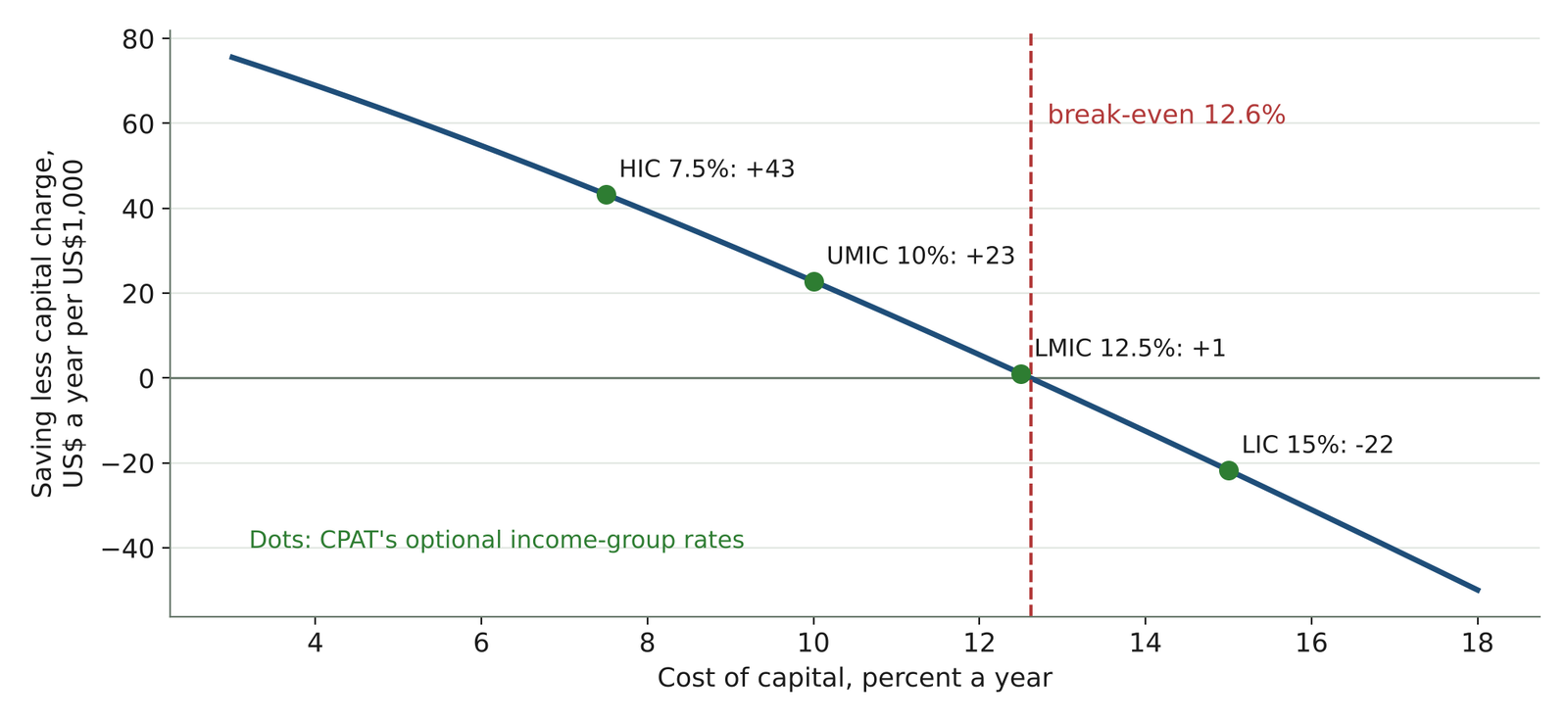
2.Source/make_figures.py).
4.3 What the lenses show
At market rates the world gains from its climate investment, but developing countries barely do. Table 1 applies the lenses to one year’s investment at the 2030 levels reported by the expert group, with the same stylized savings rate for every group, so that the differences come from the cost of capital alone. It is an illustration of scale, not an estimate: with one savings rate, it is Proposition 1 applied to three numbers.
2.Source/investment_lenses.py).
| Group (market rate / high case) | Investment, 2030 | Charge, market rate | Net, market rate | Net, high case | Charge, 6% | Net, 6% |
|---|---|---|---|---|---|---|
| Advanced economies (5.5% / 7%) | 2,750 | 205 | 161 | 130 | 215 | 151 |
| China (6% / 8%) | 1,350 | 106 | 74 | 53 | 106 | 74 |
| Developing, excluding China (10.5% / 15%) | 2,400 | 275 | 45 | −52 | 188 | 131 |
| World | 6,500 | 585 | 279 | 131 | 508 | 356 |
In developing countries the margin is thin and turns negative in a stress. At 10.5 percent, $2.4 trillion of investment earns $45 billion a year more than it costs to finance; at 15 percent it loses $52 billion. Financing at 10.5 rather than 6 percent costs $87 billion a year more for each year’s investment, and the penalty accumulates as vintages build up. At 6 percent the same investment earns $131 billion. Co-benefits widen the gap further: in SISEPUEDE’s Latin American results, avoided pollution and other health, safety and productivity gains ($1.5 trillion) exceed the fuel savings ($0.9 trillion), and counting them raises the net benefit from $0.7 trillion to $2.7 trillion (Kalra et al. 2023).
The gap between lens (a) and lens (c) is the case for public finance, and the series’ de-risking papers are tools for closing it. A private investor in a developing country sees a thin margin or a loss; society sees a large gain. Three instruments bridge the gap. Pricing carbon and air pollution turns co-benefits into revenue, which is CPAT’s home ground. Lending on concessional or multilateral terms substitutes a lower rate for the market rate. And cutting the risk premium in equation 4 lowers the WACC itself: guaranteeing the power purchase contract rather than the debt removes payment risk (Stretton 2026d), and refinancing operating plants’ senior debt through pooled, tranched securities at a blended cost of about 5.65 percent, against single-stage finance at 10 percent, cuts the cost of solar power by about a fifth (Stretton 2026c). In the terms of Proposition 1, these instruments move a country from above \(r^*\) to below it. The extension tells a ministry how much each point is worth: about $36 billion a year, near 6 percent, for each year of the $4.8 trillion of clean energy investment the expert group projects for 2030 (Bhattacharya et al. 2024). The IEA’s comparable figure for emerging and developing economies alone is about $150 billion a year of financing costs per point, on their whole clean energy capital stock rather than one year’s investment (International Energy Agency 2024).
A high cost of capital also changes what gets built. Low-carbon technologies are more capital-intensive than fossil plants, so a high cost of capital favors fossil fuels and a country with dear capital needs a higher carbon price to reach the same decarbonization (Hirth and Steckel 2016; Ameli et al. 2021). Running CPAT’s logit investment choice with country rates from equation 4 makes the physical needs in equation 1 respond to finance.
5 Extension B: the efficiency of public spending
5.1 The rule
For each candidate use of public money, compare what people get with what the budget really pays. Let \(W_j\) be the present value of benefits of measure \(j\) to everyone other than the budget, net of their own costs, and \(F_j\) the present value of its net cost to the budget, after revenue that comes back. Then
\[ \mathrm{ENPV}_j = W_j - F_j, \qquad \mathrm{MVPF}_j = \frac{W_j}{F_j}, \qquad NB_{\lambda,j} = W_j - \lambda F_j, \tag{7}\]
where ENPV is the economic net present value, MVPF is the marginal value of public funds (Hendren and Sprung-Keyser 2020) and \(\lambda\) is the marginal cost of public funds: the cost to the economy of raising one more dollar of tax. Fund measure \(j\) if \(\mathrm{MVPF}_j > \lambda\), equivalently \(NB_{\lambda,j} > 0\). If \(F_j \le 0\) the measure pays for itself and is funded whenever \(W_j \ge 0\); the binding problem is then financing, not value. When the budget binds, rank by MVPF.
The cost of public funds is about 1.2 in developing countries, and higher where taxes distort more. For 38 African countries, raising a marginal dollar through the existing mix of five taxes costs on average $1.20, and $1.10 through each country’s cheapest instrument, often the value added tax (Auriol and Warlters 2012). For proportional tax changes in Scandinavian and northern continental European welfare states, where the participation margin matters, estimates center around 2 (Kleven and Kreiner 2006). The extension defaults to 1.2, uses 1.1 where the marginal tax is value added tax, and applies 1.5 to 2.0 as a stress where the macro-fiscal and debt models say the country cannot borrow more.
Proposition 2 (the rule nests World Bank practice and prices revenue returns at \(\lambda\)). (a) With \(\lambda = 1\) and no budget limit, \(NB_{\lambda,j} = \mathrm{ENPV}_j\), the usual economic net present value test. (b) Shifting a dollar of present value from beneficiaries to the budget, for example by keeping part of a fuel saving in the utility, leaves \(\mathrm{ENPV}_j\) unchanged and raises \(NB_{\lambda,j}\) by \(\lambda - 1\).
Revenue returns belong in the denominator, not the numerator. A user fee is a transfer in economic analysis; counting it as a benefit as well as a saving double-counts. But every dollar the budget recovers saves \(\lambda\) dollars of taxation, not one. The same logic puts CPAT’s pricing policies on the spending ladder. A carbon tax or fuel subsidy reform raises money at a low welfare cost per dollar, so it is the natural first source of funds. A spending measure that a price could achieve more cheaply is flagged “price first”: with costly public funds, the best subsidy is smaller than the gap between social and private returns, and smaller still when most subsidized units would have happened anyway, whereas a tax raises money on those same units. Paper 6.1 shows how to measure what such prices cut, as a Total Effective Carbon Price (Stretton 2026e).
5.2 Five corrections between a project’s value and its claim on the budget
First, public money pays only the gap the private sector will not cover. The investor’s net present value is computed at the market WACC and private prices, including taxes. For a purely public asset the budget pays the full cost; for a viability-gap measure it pays \(\max(0, -NPV^{priv}_j)\); for utility and contracted routes it pays nothing up front and carries a contingent liability; for purely private investment it pays nothing. Benefits are scaled by an additionality share \(a_j\), the part that would not have happened without the measure.
Second, money spent is not capital created. Pritchett (2000) showed that cumulated public investment spending is a poor measure of public capital. The IMF estimates the average public investment efficiency gap, the shortfall of outcomes from what the same spending could buy, at about 30 percent across 134 countries: 40 percent in low-income developing countries, 27 percent in emerging markets and 13 percent in advanced economies. Stronger public investment management could close up to two-thirds of the gap (International Monetary Fund 2015). The extension carries an efficiency \(s_j\), the share of public spending that becomes effective capital, and an execution rate \(e_j\), the share of the budget actually spent:
\[ C^{\mathrm{eff}}_j = C_j\Big[(1-\pi_j) + \frac{\pi_j}{s_j}\Big], \qquad K^{\mathrm{eff}}_{j,t} = (1-\delta_j)K^{\mathrm{eff}}_{j,t-1} + s_j\, e_j\big(I^{\mathrm{plan}}_{j,t} + \mathrm{backlog}_{j,t-1}\big), \tag{8}\]
where \(\pi_j\) is the public share of the capital cost and \(\delta_j\) the depreciation rate. Efficiency raises the cost of a unit of public asset; execution delays benefits but loses no money, because unspent appropriations stay in the budget. This is the efficiency-adjusted public capital of the growth and debt-investment-growth literature (Gupta et al. 2014; Berg et al. 2012). The haircut applies once: never also to unit costs taken from the country’s own outturns, which already contain its inefficiency.
Third, efficiency frontiers convert into parameters. Frontier studies measure how far each country’s health and education outcomes fall short of the best achieved for the same spending, across 140 countries (Herrera and Pang 2005) and across 38 African countries, which score lower on average than Asian and Latin American ones (Gupta and Verhoeven 2001). Outcomes of measures costed from international norms are scaled by the country’s score; those costed from local outturns are not.
Fourth, capital and current spending go on one footing. Each capital outlay becomes an equivalent annual cost with its recurrent costs added:
\[ \mathrm{EAC}_j = K_j\,\mathrm{CRF}(r, n_j) + r^{rc}_j K_j, \tag{9}\]
where \(r^{rc}_j\) is the recurrent-cost coefficient: operations, maintenance and staffing per dollar of capital a year. Recurrent costs are large in aggregate: on top of investment of 4.5 percent of GDP, keeping infrastructure in low- and middle-income countries running adds 2.7 percent of GDP a year (Rozenberg and Fay 2019). By sector the coefficients differ widely; as illustrative values, the extension uses about 1 to 2 percent for solar and single digits for roads, and 10 to 20 percent for clinics and schools because of staffing. The rate \(r\) is the social rate for the economic view, the government’s borrowing rate for the fiscal view, and the market WACC for private and contracted routes. Underfunded maintenance is a measure in its own right, funded before new building of the same asset class, because unfunded recurrent costs are one of the main ways public capital in low-income countries loses value (Adam and Bevan 2014).
Fifth, the financing route changes the fiscal ledger, the debt statistics and the liabilities, and the extension runs each measure under six of them. These are a commercial loan, a concessional loan, a utility balance sheet, an independent producer under a power purchase agreement (PPA) with or without a guarantee, a viability-gap contract and a grant. The yearly net fiscal flow is
\[ F_t = \mathrm{capex}_t - \mathrm{loans}_t + DS_t + OM^{pub}_t + PPA_t + SUB_t - FEE_t - \theta\, SAV_t + XL_t - PIG_t + \mathbb{E}[\mathrm{CALL}_t], \tag{10}\]
with debt service \(DS\), public operation and maintenance \(OM^{pub}\), contract payments \(PPA\), subsidies \(SUB\), fees \(FEE\), avoided fuel cost \(SAV\) of which the budget or state utility keeps a share \(\theta\), fuel excise lost \(XL\), earmarked corrective revenue \(PIG\), and expected guarantee calls. For a PPA the tariff and the liability are
\[ T = \frac{\big(K + PV_w(\mathrm{rep})\big)\,\mathrm{CRF}(w, n) + OM}{E}, \qquad L^{PPA} = \sum_{t=1}^{n} \frac{T E}{(1+i_g)^t}, \tag{11}\]
where \(w\) is the producer’s WACC, \(\mathrm{rep}\) mid-life replacements, \(E\) annual energy and \(i_g\) the government’s borrowing rate.
Proposition 3 (tenor is not price). (a) If a loan’s rate equals the government’s borrowing rate \(i_g\), the present value of its debt service at \(i_g\) equals the principal whatever its tenor, so the fiscal net present value at \(i_g\) does not depend on tenor; tenor changes only the timing of cash. (b) If budget costs are discounted at a social rate below the loan rate, the present value of debt service rises with tenor, so a rule with one constant \(\lambda\) ranks the shorter loan above the longer one. (c) Only a cost of public funds \(\lambda_t\) that is higher in cash-short years can reverse that ranking.
Proposition 4 (a power purchase agreement is debt in disguise). Let the producer’s WACC \(w\) exceed \(i_g\) and the PPA be take-or-pay over the asset life. (a) Without mid-life replacements, \(L^{PPA} > K + PV_{i_g}(OM)\): the committed payments, valued at the government’s rate, exceed the cost of building and running the plant. (b) With replacements, \(L^{PPA} > K + PV_{i_g}(OM) + PV_{i_g}(\mathrm{rep})\) if and only if \(\big(K + PV_w(\mathrm{rep})\big)\,\mathrm{CRF}(w,n)/\mathrm{CRF}(i_g,n) > K + PV_{i_g}(\mathrm{rep})\). The excess is the financing premium the country pays for keeping the asset off its headline debt.
Debt rules see only part of this. The proofs are in Appendix A. In the joint IMF and World Bank framework for low-income countries, once the stock of public-private partnership capital exceeds 3 percent of GDP, a stress test adds 35 percent of that stock to public debt (International Monetary Fund and World Bank 2017). Public-private partnerships do not free public funds; any case for them rests on efficiency gains large enough to beat the financing premium (Engel et al. 2013).
5.3 From measures to a portfolio
Ranking by MVPF within an affordable envelope gives an allocative frontier across sectors. Measures are ranked by MVPF and cumulative fiscal cost is plotted against cumulative value. Mutually exclusive variants of one measure keep only the efficient ones; indivisible projects need a knapsack:
\[ \max_{x} \sum_j x_j\, NB_{\lambda,j} \quad \text{s.t.} \quad \sum_j x_j F_{j,t} \le E^{*}_t \;\;\forall t, \qquad \sum_{j \in g} x_j \le 1 \;\;\forall g, \qquad \sum_j x_j I_{j,t} - I_{t-1} \le \Delta I^{\max}, \tag{12}\]
where \(x_j\) is 1 if measure \(j\) is funded (or a share if divisible), \(g\) indexes families of exclusive variants, \(E^*_t\) is the fiscal envelope that the macro-fiscal and debt models say is affordable, and \(\Delta I^{\max}\) caps the speed of scale-up, which matters most where absorptive capacity is low. Climate measures sit on the same ladder as health, education, roads, water and cash transfers, each on a “sector card” with a unit cost, outcome per dollar and recurrent-cost coefficient, sharing one discount rate, value of a statistical life and shadow price of carbon. A cash transfer, with an MVPF near 1, is the benchmark to beat. The cut-off MVPF is itself a diagnostic: well above \(\lambda\) means the envelope is too tight; below it means the envelope is too loose.
The chosen portfolio then goes back to the macro-fiscal models, which return the envelope and \(\lambda\). Public capital by sector, its efficiency, the financing shares and the contract liabilities pass to the debt-investment-growth and debt sustainability models of paper 6.5 (Stretton 2026g), which return the debt path and the affordable envelope. Non-market benefits such as health enter \(W\) but never GDP, so the macro model does not count them twice.
6 A worked example: a small island caught in the oil trap
The example is stylized: an island of $2 billion GDP and 85 percent public debt that makes almost all its 300 gigawatt-hours of power from imported diesel. It replaces 30 percent of its diesel generation with 60 megawatts of solar and a 120 megawatt-hour battery costing $120 million (6 percent of GDP). Unit costs are anchored to public data with an island premium: solar at $1,200 a kilowatt against a 2024 global average of $691 (International Renewable Energy Agency 2025). Diesel generation avoided costs $0.228 a kilowatt-hour at a Brent price of $80 a barrel, so the plant saves $20.5 million a year (1 percent of GDP). The social rate is 6 percent, the government borrows at 8 percent, \(\lambda\) is 1.2, and the budget or state utility keeps half the fuel saving (\(\theta = 0.5\)), passing the rest to consumers. Appendix B lists every parameter.
Before financing, the plant is excellent. Its levelized cost at 6 percent is $0.134 a kilowatt-hour against the $0.228 it displaces, its economic net present value is $108 million, and it stays positive down to oil at about $22 a barrel. SISEPUEDE’s method, or a standard World Bank appraisal, would stop here.
The plant passes the public-money test on every route, but the only commercial loan breaks the budget’s cash flow. The island can borrow commercially at 8 percent for seven years. Debt service and upkeep come to $24.8 million a year against $20.5 million of fuel saved, of which the budget keeps half: the net cash flow to the budget is −$14.6 million a year for seven years, $102 million in all, and even if the budget kept every dollar saved it would still run $4.4 million short each year. Headline debt rises from 85 to 91 percent of GDP on day one. Yet the MVPF on this route is 4.18 and the net benefit at \(\lambda = 1.2\) is $93 million. Table 2 sets the five financing routes side by side, and Figure 2 shows the cash and the liabilities.
2.Source/sids_worked_example.py).
| R1a: loan 8%, 7 yr | R1b: loan 8%, 25 yr | R2: concessional 1.5%, 30 yr | R3: PPA, WACC 11% | R4: PPA, WACC 8.5%, guaranteed | |
|---|---|---|---|---|---|
| Year-1 payment for the plant ($m) | 24.8 | 13.0 | 3.6 | 16.7 | 14.2 |
| Year-1 net cash to budget ($m) | −14.6 | −2.8 | +6.6 | −6.4 | −4.0 |
| Island ENPV ($m) | 100 | 85 | 165 | 49 | 80 |
| MVPF | 4.18 | 2.82 | pays for itself | 1.59 | 2.55 |
| \(NB_{1.2}\) ($m) | 93 | 75 | 172 | 32 | 69 |
| \(NB\) with liquidity premium ($m) | 28 | 63 | 197 | 3 | 51 |
| Fiscal NPV at 8% ($m) | −38 | −38 | +33 | −69 | −43 |
| Headline debt added (% of GDP) | 6.0 | 6.0 | 6.0 | 0 | 0 |
| PV of PPA payments at 8% / capital cost | — | — | — | 1.48 | 1.27 |
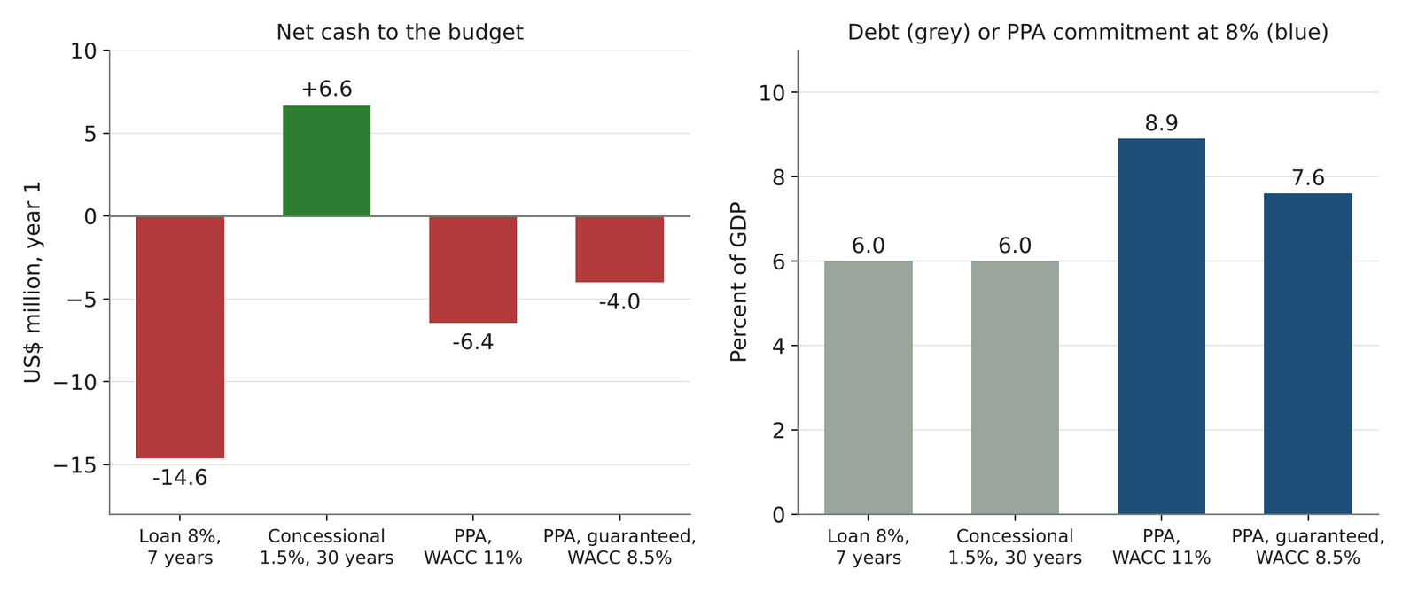
2.Source/make_figures.py).
The trap is a liquidity and debt-statistics problem, not a solvency problem. The short tenor creates the cash gap, the 8 percent rate sets the fiscal cost, and the debt rule penalizes the gross liability rather than the self-financing asset behind it. Tenor eases the first but not the second: the seven-year and 25-year loans have the same fiscal net present value at 8 percent, −$38 million (Proposition 3). At a constant \(\lambda\) of 1.2 the short loan even ranks higher ($93 million against $75 million), because the island pays the two-point spread over the social rate for fewer years. Only when \(\lambda\) rises to 2 in the cash-short years does the ranking flip, to $63 million against $28 million. A tool with one constant cost of public funds cannot see the trap.
Concessional finance wins on every count, where it exists. A 30-year loan at 1.5 percent with five years’ grace has a grant element of 48 percent at 6 percent, puts $6.6 million a year into the budget from the first year, and pays for itself in MVPF terms. It still adds 6 percent of GDP to headline debt. The constraint is volume, not merit.
A PPA turns capital into an annual payment below the fuel bill, but it does not remove the liability. At an 11 percent WACC the tariff is $0.186 a kilowatt-hour, and at 8.5 percent with a World Bank or Multilateral Investment Guarantee Agency guarantee $0.159, both below the $0.228 avoided cost. Neither adds headline debt, and both narrow the budget’s year-one gap, to $6.4 and $4.0 million. But the present value of the committed payments at 8 percent is 1.48 times the capital cost without a guarantee and 1.27 times with one, 8.9 and 7.6 percent of GDP, more than the 6 percent of GDP of debt kept off the books. Against the full cost of building and running the plant valued at 8 percent, the excess is about $31 million without a guarantee and $5 million with one (Proposition 4); so the guaranteed PPA is a fair second-best to sovereign borrowing. The unguaranteed PPA halves the island’s net benefit and fails at \(\lambda = 2\), at oil of $60, or with capital costs 30 percent higher. The guarantee, cutting the producer’s cost of capital by 2.5 points, is worth about $31 million to the island, a quarter of the plant’s cost.
Who keeps the fuel saving decides the MVPF but not the economic value. Moving \(\theta\) from 0 to 1 leaves each route’s economic net present value unchanged but raises the seven-year loan’s MVPF from 1.61 to “pays for itself” (Proposition 2, part b); above a \(\theta^*\) of 0.37 for the concessional route and 0.62 to 0.81 for the others, the plant finances itself. Tariff design is a fiscal lever worth \(\lambda - 1\) per dollar.
Carbon at the shadow price adds $47 to 93 million of present value to every route but does not reorder them, because all five displace the same diesel.
7 Country runs: Kenya, Uganda and St Lucia
Run for three countries, the investment-needs extension puts 2030 mitigation investment at 4 to 5 percent of GDP, and the lens decides whether the increment is a cost or a gain. Table 3 reports the tool’s 2030 results for Kenya, Uganda and St Lucia (Mitigation Investment Needs Model 2026). The tool shares the expert group’s totals among countries by physical drivers from CPAT and by GDP, so country values are allocations, not bottom-up estimates; they are illustrative results from the tool, not official estimates.
2.Source/country_runs.py.
| Kenya | Uganda | St Lucia | |
|---|---|---|---|
| GDP, 2030 (US$ billion) | 155.7 | 87.5 | 2.9 |
| Total investment (% of GDP) | 4.7 | 4.0 | 4.4 |
| Incremental investment (% of GDP) | 1.1 | 1.0 | 1.1 |
| Market cost of capital (%) | 9.7 | 8.5 | 10.5* |
| Incremental cost, lens (a), market rate (US$ million a year) | 120 | 56 | −1.2 |
| Incremental cost, lens (b), 6% | 68 | 39 | −2.3 |
| Incremental cost, lens (c), 6% and local co-benefits | −7 | −3.5 | −3.0 |
| Total investment after the delivery haircut (US$ billion) | 8.3 (7.2) | 4.3 (3.5) | 0.145 (0.126) |
In Kenya and Uganda the increment is a net cost at market rates and at 6 percent, and pays only when cleaner air is counted; in St Lucia it pays at any rate. Kenya’s incremental investment costs $120 million a year more than it saves at its market rate, $68 million at 6 percent, and becomes a small gain with co-benefits. St Lucia, which burns imported diesel for almost all its power, saves more than the capital charge even at 10.5 percent, as the stylized island does. Uganda’s observed cost of capital, 8.5 percent, is far below the 15 percent that CPAT’s income-group option would assign a low-income country; the choice of setting alone can turn the stylized asset of Proposition 1 from a loss into a gain. The delivery haircut matters as much: it raises Uganda’s investment need by $0.8 billion, about a fifth, because its public investment efficiency gap is 36 percent.
A full SISEPUEDE run for Uganda shows what replaces the share-of-GDP fallback, and how little of its value a budget can see. In the October 2025 run, the net-zero strategy carries $259 billion of undiscounted technical cost over 2025–2050 against $675 billion of benefits, a net present value of $161 billion at 6 percent and $116 billion at 8.5 percent (SISEPUEDE 2025). Two strategies under Uganda’s nationally determined contribution score $185 billion and $90 billion at 6 percent. Technical cost rises from 1.4 percent of the run’s GDP in 2030 to 3.8 percent in 2050. But only the fuel, system-cost and technical-savings lines are cash that a budget, a utility or the balance of payments would see: $119 billion, 18 percent of the net-zero benefits and under 3 percent in the two other strategies. The rest is health, indoor air, crops and water quality. And power is only 6 percent of the technical cost; wastewater, buildings, livestock, solid waste and sanitation dominate. A spending test on this run would therefore find large values of \(W\) and small cash returns in \(F\) (Section 5): strong cases for public money, financed mostly by tax rather than by the savings they generate.
8 Validation, limits and use
The extensions are built to reproduce existing results when their new parameters are switched off. With \(\lambda = 1\), no haircuts and no budget limit, the spending layer must return the economic net present value of a standard appraisal (Proposition 2, part a), and with the investment lenses at a common rate it must return the capital charge of equation 3. With financiers resident, the island’s ENPV must equal the financing-neutral ENPV on every route; the worked-example code asserts this, along with the identity that a loan’s debt service discounted at its own rate equals the principal. These are the same regression tests that paper 5.2 applies to the core model (Stretton 2026b).
The strongest objection is that the lenses only restate a discount-rate sensitivity. With one savings rate for every group, Table 1 is indeed Proposition 1 applied to three numbers. The answer is that the lenses separate two jobs a single rate is asked to do. The market rate prices finance and can be changed by policy: guarantees, pooling, concessional terms. The social rate values time and cannot. Reporting both, with co-benefits beside them, tells a ministry how much of the gap between what investors see and what society gets is a financing problem it can buy down, and at what price per point.
The weakest parameters are the savings, co-benefit and abatement rates per dollar, and they matter most. The stylized 13.3 cents of savings per dollar is calibrated to one region’s results. The country runs rest on the investment-needs tool’s own savings and co-benefit rates per dollar, which are calibrated, not observed. Each should be replaced by a country run of SISEPUEDE, as for Uganda, or by CPAT’s own fuel savings, before any number goes into a budget document.
The country cost of capital is the most influential input and the least measured. Observed costs of capital for renewable projects exist for a few dozen economies (St Lucia is not one). CPAT’s default country table rests on a calculator of risk-free rates, country risk premiums and spreads plus a technology premium set by judgment; sovereign spreads overstate project risk where contracts are guaranteed and understate it where they are not. An open table of the cost of capital by country and technology, with its sources, is the first job.
Several simplifications bias the worked example in known directions. Nominal rates applied to constant-price flows overstate financing costs; take-or-pay is an upper bound on the PPA liability; the guarantee is unpriced; and no delivery haircut is applied to the public routes. The extension uses an end-of-year capital recovery factor and CPAT a year-zero one; Proposition 1’s break-even rate is 12.6 percent under the first and 14.8 percent under the second, so the two must be aligned before results are compared.
For a ministry, the extensions answer three questions in order. First, how much clean capital a policy package calls for, by sector, and how much of it the public sector must carry: run CPAT, take its capacity changes, and apply equation 1 to equation 6 at the country’s WACC and at 6 percent. Second, which of the public measures pass the budget test: tag each by payer and financing route, apply the five corrections and rank by MVPF against \(\lambda\). Third, how to finance the survivors: compare routes on the fiscal ledger, the debt statistics and the contract liabilities, with a time-varying \(\lambda\) where cash is short. The method uses public data and the outputs CPAT and SISEPUEDE already produce.
9 Conclusion
A carbon price model that cannot price capital tells a finance ministry half of what it needs. Extending CPAT to investment needs shows that the cost of capital, not the size of the bill, decides whether developing-country climate investment pays its way: a typical clean asset that pays its way at 6 percent breaks even at 12.6 percent, the rate CPAT’s income-group option gives lower-middle-income countries, while the economic case is strong everywhere. Which of CPAT’s two cost-of-capital settings a team uses, and which capital-recovery convention, can each move that verdict. Extending CPAT to the efficiency of public spending shows that the budget’s problem is often not value but liquidity, debt statistics and hidden contract liabilities, and that a single cost of public funds cannot see a cash trap. The country runs show the same pattern on tool results: in Kenya and Uganda the increment pays only when co-benefits are counted, and in Uganda’s SISEPUEDE run under a fifth of the net-zero benefits reach the budget as cash. The main limitation is that the savings per dollar and the costs of capital that drive every number are calibrated on one region and a few dozen observations. The next step is an open country-by-technology table of the cost of capital and more SISEPUEDE runs outside Latin America, so that the lenses rest on country data rather than stylized ratios.
Downloads
References
10 Appendix A. Proofs
Proposition 1. Per dollar of capital, \(N^F = b - \mathrm{CRF}(\mathrm{WACC}, n)\). \(\mathrm{CRF}(r,n)\) is continuous and strictly increasing in \(r\) for \(n > 1\): it is the level payment that repays one dollar over \(n\) years, and the present value of any fixed payment stream strictly falls as \(r\) rises, so a larger payment is needed. As \(r \to 0\), \(\mathrm{CRF} \to 1/n\); as \(r \to \infty\), \(\mathrm{CRF} \to \infty\). So if \(b > 1/n\) there is a unique \(r^* > 0\) with \(\mathrm{CRF}(r^*, n) = b\), and \(N^F > 0\) if and only if \(\mathrm{WACC} < r^*\). Numerically, \(\mathrm{CRF}(0.126, 25) = 0.133\) (investment_lenses.py). With savings from year zero, as in CPAT’s levelized cost, the condition becomes \(\mathrm{CRF}(r^*, n)/(1+r^*) = b\), with \(r^* = 14.8\) percent.
Proposition 2. (a) Substitute \(\lambda = 1\) into \(NB_{\lambda,j} = W_j - \lambda F_j\). Without a budget limit the funding rule is \(NB > 0\) for each measure independently, which is the ENPV rule. (b) A transfer of \(\Delta\) in present value from beneficiaries to the budget changes \(W_j\) by \(-\Delta\) and \(F_j\) by \(-\Delta\). So \(\mathrm{ENPV}_j = W_j - F_j\) is unchanged and \(NB_{\lambda,j}\) changes by \(-\Delta + \lambda\Delta = (\lambda - 1)\Delta\).
Proposition 3. (a) A level annuity loan of principal \(K\) at rate \(i\) over \(n\) years pays \(K\,\mathrm{CRF}(i,n)\) a year, whose present value at \(i\) is \(K\) for any \(n\). With \(i = i_g\), the loan’s contribution to the fiscal net present value at \(i_g\) is \(K - K = 0\) for every tenor. (b) At a social rate \(r < i\), the present value of the debt service is \(K\,\mathrm{CRF}(i,n)/\mathrm{CRF}(r,n)\). The ratio \(\mathrm{CRF}(i,n)/\mathrm{CRF}(r,n)\) rises with \(n\) when \(i > r\), from \((1+i)/(1+r)\) at \(n = 1\) toward \(i/r\) as \(n \to \infty\), because the longer the loan the longer the spread is paid. All other terms of \(F_j\) are independent of tenor, so with constant \(\lambda\), \(F_j\) is larger and \(NB_{\lambda,j}\) smaller for the longer tenor. (c) With \(\lambda_t\) higher in the early years, the short loan’s front-loaded payments are weighted more heavily, which can reverse the ranking; Table 2 gives an instance.
Proposition 4. Under take-or-pay the committed payment each year is \(TE = (K + PV_w(\mathrm{rep}))\,\mathrm{CRF}(w,n) + OM\). A level payment \(X\) over \(n\) years has present value \(X/\mathrm{CRF}(i_g,n)\) at \(i_g\). So \(L^{PPA} = (K + PV_w(\mathrm{rep}))\,\mathrm{CRF}(w,n)/\mathrm{CRF}(i_g,n) + PV_{i_g}(OM)\). Subtracting \(K + PV_{i_g}(OM) + PV_{i_g}(\mathrm{rep})\) gives part (b) directly. For part (a), set \(\mathrm{rep} = 0\): because CRF is strictly increasing in the rate, \(w > i_g\) implies \(\mathrm{CRF}(w,n)/\mathrm{CRF}(i_g,n) > 1\), so \(L^{PPA} > K + PV_{i_g}(OM)\). With replacements the inequality can fail, because a replacement is discounted at \(w\) inside the tariff and at \(i_g\) outside it; a large late replacement and a WACC barely above \(i_g\) give a counterexample. In the worked example it holds: the excess is about $31 million at an 11 percent WACC and $5 million at 8.5 percent.
11 Appendix B. Code and parameters
2.Source/investment_lenses.py prints Table 1 and the break-even rate. 2.Source/sids_worked_example.py (Python 3, NumPy, pandas) prints Table 2, the switching values and the sensitivities, writes sids_worked_example_results.csv and sids_worked_example_sensitivity.csv, and asserts the accounting identities described in Section 8. 2.Source/make_figures.py draws Figure 1 and Figure 2. 2.Source/country_runs.py extracts Table 3 and the Uganda figures from the two tools’ files.
Worked-example parameters (all stylized unless a source is given): demand 300 GWh a year, all diesel; GDP $2.0 billion; public debt 85 percent of GDP; 60 MW solar at $1,200/kW (2024 global average $691/kW from International Renewable Energy Agency (2025), times an island premium); 120 MWh battery at $350/kWh, replaced in year 15 at 60 percent of cost; integration 5 percent of capital; operation and maintenance 1.5 percent of capital a year; capacity factor 18 percent with 95 percent delivered; 25-year life; Brent $80 a barrel (sensitivities $60 and $110), diesel crack $25 a barrel, island delivery premium $0.15 a liter, 3.9 kWh per liter, non-fuel variable cost $0.02/kWh; fuel excise on power diesel zero; \(\theta = 0.5\) (sensitivities 0 and 1); emission factor 2.68 kg CO₂ per liter; shadow price of carbon $40 a ton in 2020 rising 2.25 percent a year, the low end of the High-Level Commission’s range ($50 in 2030), with a high path double that (High-Level Commission on Carbon Prices 2017); social rate 6 percent; government rate 8 percent; \(\lambda = 1.2\) (stress 2.0; liquidity case 2.0 in years 1–7); concessional loan 1.5 percent, 30 years, 5 years’ grace; producer WACC 11 percent, or 8.5 percent with a guarantee; 25-year PPA treated as take-or-pay; all financiers non-resident; debt framework stress of 35 percent of the public-private partnership capital stock once that stock exceeds 3 percent of GDP (International Monetary Fund and World Bank 2017).
Footnotes
The extensions began as the author’s design notes on global investment needs and on the efficiency of public spending, written to sit beside the Climate Policy Assessment Tool and the open SISEPUEDE model. CPAT’s settings are checked against the public documentation (CPAT Team 2024) and the public CPAT-AI repository (CPAT-AI Project 2026). The island example is stylized. The country runs are illustrative results from the investment-needs tool and from a SISEPUEDE run for Uganda, not official estimates. Errors are the author’s own.↩︎