Are CPAT’s Price Elasticities Right?
A Check Against the Evidence
The Climate Policy Assessment Tool, used by the International Monetary Fund and the World Bank to estimate what carbon prices and fuel subsidy reforms do, turns every price change into emission cuts through a table of elasticities. This paper checks the tool’s default long-run own-price elasticities, fuel by fuel and sector by sector, against meta-analyses, reviews and well-identified studies, keeping the tool’s own calibration source apart from independent evidence. Eight of ten main fuel-sector pairs lie within the published range, and for six of them the default is less elastic than the median estimate. Two values built from thin sector evidence are too high: diesel in industry and gasoline in services, at about −1.05 against estimates of −0.25 to −0.84. Road gasoline, at −0.64, matches uncorrected averages but is twice the estimate corrected for publication bias. The larger problem is structural: the tool applies the full long-run response within one year, which overstates five-year responses by about 30 to 110 percent, and it has almost no cross-price terms. The errors matter for estimated emission cuts and early revenue much more than for the Total Effective Carbon Price. The paper sets out a repeatable validation protocol.
price elasticity, energy demand, meta-analysis, publication bias, carbon pricing, model validation
Working paper, version 0.2, October 2026. Stephen J. Stretton, writing in a personal capacity. The views expressed are the author’s own and do not represent those of any institution with which he is or has been affiliated. A short version for policy makers is Climate Fiscal Policy Brief No. 5.4. Companion paper to the public CPAT-AI repository (https://github.com/cpmodelai/cpat_ai).1
1 Executive summary
Policy brief (short version) → · Download this paper (pdf) · Slides (pdf)
A carbon-pricing model’s answer is set mostly by its price elasticities. The Climate Policy Assessment Tool (CPAT), built by the International Monetary Fund (IMF) and the World Bank, tells finance ministries how much a carbon tax or a fuel subsidy reform will cut emissions and raise revenue. It does so by applying, to each fuel in each sector, a number saying how much use falls when the price rises: the price elasticity. Double the elasticity and the estimated cut doubles. CPAT’s own sensitivity tests show that the elasticities move its answers more than any other parameter: varying them by two standard deviations moves the cut in G20 emissions from a $75 carbon tax from 29 percent to anywhere between 7 and 39 percent.
This paper checks CPAT’s default elasticities against the published evidence, pair by pair. It compares the tool’s long-run elasticities for ten main fuel-sector pairs with meta-analyses (studies that pool hundreds of estimates), reviews of developing-economy evidence and well-identified single studies, every number checked against its source. It keeps apart the figures CPAT was calibrated to, so that the tool is not tested against itself.
Most defaults are consistent with the evidence, and most are on the cautious side. Eight of ten pairs lie inside the range of published estimates. For six, CPAT’s value is less elastic than the median estimate: electricity used by industry, for example, is −0.44 in CPAT against a median of −0.69. Two values are clearly too high. Diesel in industry (−1.06) and gasoline in services (−1.04) lie beyond every estimate for their fuels, which run from −0.25 to −0.84; both come from applying sector adjustments estimated on few studies to fuels with almost no sector evidence. Electricity in services (−0.70) sits at the elastic edge of the range.
For road fuels, publication bias is the bigger question. Researchers rarely publish estimates that look too small or have the wrong sign, so published averages overstate the true response. Correcting for this halves the long-run gasoline elasticity, from −0.69 to −0.31; in 32 countries that subsidize fuel, the long-run elasticity is −0.25. CPAT’s −0.64 for road gasoline matches the uncorrected averages but is twice the corrected one.
The timing of the response matters more than its size. CPAT applies the full long-run response in the year the price changes. The evidence says it takes a decade, because people change how much they drive or heat within a year or two but replace cars, boilers and machines only slowly. Under standard adjustment speeds, only about a fifth of the long-run response has happened after one year and about 60 percent after five. Five years out, CPAT’s response is 45 to 72 percent larger than the gradual one, and between about 30 and 110 percent under other plausible speeds. CPAT’s developers list the missing short-run distinction as a known issue. The tool also has almost no cross-price effects, so a tax on coal does not move industry from coal to gas or electricity.
These errors matter for emission cuts and near-term revenue, much less for comparing countries. In the stylized economy of paper 6.1, CPAT’s demand elasticities more than double the cut that comes from using less energy. But the Total Effective Carbon Price, which measures a policy mix as the uniform carbon tax that would cut emissions as much, moves by only about a tenth, from $36.9 to $33.1 per tonne, because a common error largely cancels.
What to do. Model users should read CPAT’s near-term cuts and early revenue as upper bounds on the response and lower bounds on revenue, and should show a publication-bias case (road fuel elasticities halved) beside every central result. CPAT’s maintainers should bring the two outlying values into range, add separate adjustment speeds for use and for equipment, and run the eight-step validation protocol in Section 8 at every update. The policy brief gives the decisions in short.
2 Introduction
A finance ministry that asks how much a $50 carbon tax will cut its emissions gets an answer whose size is set mostly by one set of numbers: the price elasticities of energy demand. CPAT projects fuel use for each fuel and sector of the more than 180 countries it covers and moves it with prices through elasticities (World Bank and International Monetary Fund 2022; Black et al. 2022). If the elasticity for diesel in industry is twice the true value, the tool reports twice the cut from industrial diesel and overstates how fast that tax base erodes. CPAT’s own sensitivity analysis finds the price elasticities the most influential parameters it has: two standard deviations either way move the cut in G20 CO₂ emissions from a $75 carbon tax from 29 percent to between 7 and 39 percent (CPAT-AI project 2026, “Parameter Sensitivity Analysis”; Stretton 2026c). The same elasticities weight fuels in the Total Effective Carbon Price, the measure of a policy mix’s carbon-pricing effort in paper 6.1 (Stretton 2026b).
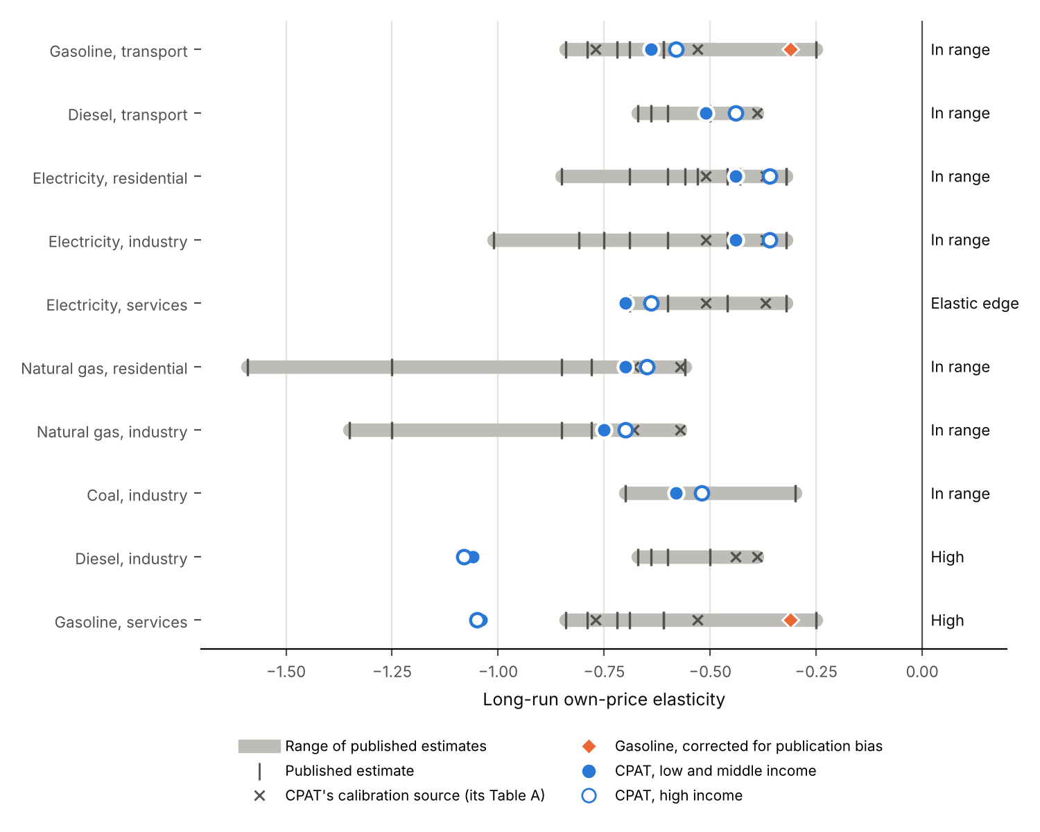
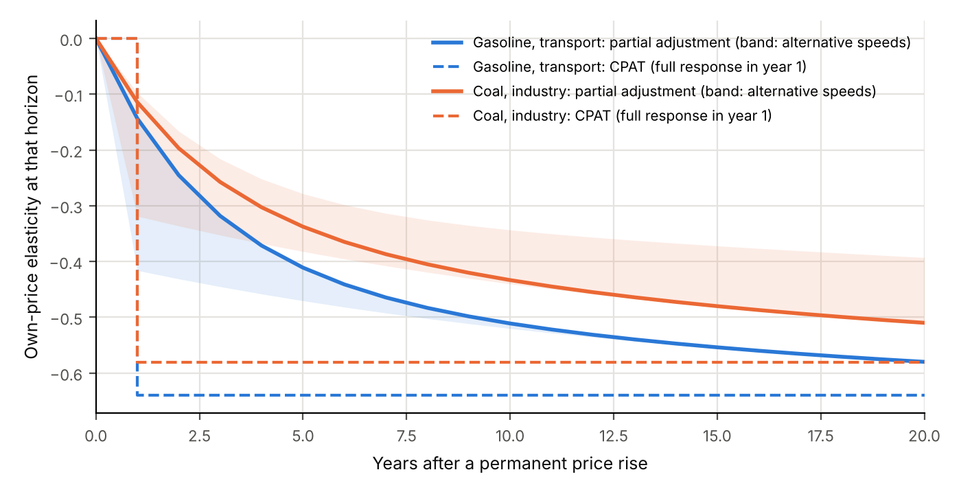
This paper asks whether CPAT’s default price elasticities are consistent with the published evidence, and what follows where they are not. The answer is that the levels are mostly consistent and often cautious, two sector values are too high, and the structure is the bigger problem. Eight of ten main fuel-sector pairs lie inside the range of published long-run estimates (Table 1, Figure 1), and for six the default is less elastic than the median independent estimate. Diesel in industry and gasoline in services, at about −1.05, lie beyond every estimate for their fuels; electricity in services, at −0.70, sits at the elastic edge. Road gasoline, at −0.64, matches the uncorrected meta-analytic means but is twice the mean corrected for publication bias, −0.31 (Havranek et al. 2012), and more than twice the long-run estimate for fuel-subsidizing economies, −0.25 (Arzaghi and Squalli 2015). The structural problems are larger. CPAT applies the full long-run response in the year the price changes; with standard adjustment speeds, only about a fifth of it has happened after one year and about 60 percent after five (Figure 2). And it applies own-price elasticities with only three cross-price terms, so it has almost no fuel switching outside power.
The closest prior work is CPAT’s own. Its documentation reports that the elasticities were calibrated to targets derived from one meta-analysis (Labandeira et al. 2017), checks the calibrated values against those targets (its Table C), and compares them with panel estimates on CPAT’s data, which found lower values for road gasoline and residential electricity (CPAT-AI project 2026). The IMF describes the result as long-run elasticities “generally between −0.5 and −0.8”, consistent with “the mid-range of the empirical literature” (Black et al. 2022). This paper adds an outside check: a register of verified estimates for each fuel and sector, kept separate from the calibration source; the benchmarks that the internal checks lack, namely estimates corrected for publication bias and estimates for fuel-subsidizing economies; bounds on the timing error; and the effect of each finding on emission cuts and on the Total Effective Carbon Price, using the demand system of paper 6.1 (Stretton 2026a). It ends with a repeatable protocol, with code in 2.Source/.
3 How CPAT turns prices into fuel use
CPAT moves each fuel’s use with income, price and an efficiency trend, one year at a time. For fuel \(f\) in sector \(s\) of country \(c\), consumption \(F\) grows from one year to the next as \[ \frac{F_{csf,t}}{F_{csf,t-1}} = \Big(\frac{1}{1+\alpha_{sf}}\Big)^{1+\epsilon_U} \Big(\frac{Y_{c,t}}{Y_{c,t-1}}\Big)^{\epsilon_Y} \Big(\frac{p_{csf,t}}{p_{csf,t-1}}\Big)^{\epsilon_U + \epsilon_F(1+\epsilon_U)}, \tag{1}\] where \(Y\) is real GDP, \(p\) the real end-user price including taxes, \(\alpha\) an autonomous efficiency gain of 0.5–1 percent a year, \(\epsilon_Y\) the income elasticity, \(\epsilon_U\) the usage elasticity (how intensively existing vehicles, boilers and appliances are used) and \(\epsilon_F\) the efficiency elasticity (how much more efficient the stock becomes) [CPAT-AI project (2026), “Fuel Consumption Dynamics”; a Covid adjustment for 2020–21 is omitted here].
The total own-price elasticity is therefore \[ \epsilon = \epsilon_U + \epsilon_F + \epsilon_U\epsilon_F . \tag{2}\] The positive product term is the direct rebound: a more efficient car is cheaper to drive, so it is driven more. CPAT’s documentation describes this term as offsetting 15 percent of the response when both margins are −0.3, “lower” than the 26–29 percent long-run rebound found for road transport in a meta-analysis of 74 studies (Dimitropoulos et al. 2018). The comparison mixes definitions. The meta-analysis measures rebound as the share of an efficiency gain taken back by more use; in equation 1 that share is \(-\epsilon_U\), which is 30–40 percent for road gasoline and diesel. On a like-for-like definition CPAT’s rebound is at or slightly above the meta-analytic value.
The defaults are set by fuel, sector and income group. The public legacy release of CPAT (version 1.0pre) holds usage elasticities for eight fuels and four end-use sectors in four income groups, and efficiency elasticities that are the same across income groups (CPAT-AI project 2026). Usage elasticities run from −0.1 to −0.7 and efficiency elasticities from −0.2 to −1.2. Every usage elasticity is 0.1 larger in magnitude in low- and middle-income countries than in high-income ones, following the finding that price elasticities are slightly higher in developing countries. The documentation says this adjustment is made “on the extensive margin”; the data put it on the usage margin (World Bank and International Monetary Fund 2022; CPAT-AI project 2026). The targets come from the meta-analysis of Labandeira, Labeaga and López-Otero, expressed as a “base (assumed transport)” plus deviations for the residential, industrial and service sectors, and “all elasticities are long-term elasticities” (World Bank and International Monetary Fund 2022). A simplified set kept with the tool’s carbon-price validation files, by fuel only, uses −0.58 for coal and liquid fuels, −0.70 for natural gas, −0.36 for electricity and −0.44 for biomass (CPAT-AI project 2026, other/tecp_and_validation).
Income elasticities follow a reverse-U in income per head. CPAT starts from 32 base income elasticities by fuel and sector, chosen so that the cross-fuel average matches sectoral energy–GDP elasticities for 132 countries (Burke and Csereklyei 2016). It then scales them with income per head along a curve inferred from Gertler et al. (2016), rising to a peak near $3,000 per head and declining toward the high-income level, calibrated so that the global average equals 0.74, the aggregate energy–GDP elasticity in Burke and Csereklyei’s 2010 cross-section (CPAT-AI project 2026; Burke and Csereklyei 2016). The comparison in Section 5.1 uses the base values.
Power generation and fuel switching sit outside equation 1. Electricity demand follows equation 1 with its own elasticities. The generation mix responds to generation costs through a conditional elasticity, −0.5 for nearly every technology and country in the elasticity-based power model, or through the engineering model’s dispatch and investment rules; the documentation recommends the average of the two for standard use (CPAT-AI project 2026). Between end-use fuels, CPAT has three cross-price elasticities: biomass with respect to LPG and kerosene in households, and gasoline with respect to diesel. A carbon tax that raises the price of coal in industry therefore cuts coal use by coal’s own-price elasticity, and nothing in the industrial block shifts that demand to gas or electricity.
The demand system of paper 6.1 gives the yardstick. In a nested constant-elasticity-of-substitution (CES) system, each sector’s fuels combine into an energy service with substitution elasticity \(\sigma_s\), and demand for the service has price elasticity \(-\eta_s\). The own-price elasticity of fuel \(f\) with cost share \(s_f\) is then \(-\sigma_s + (\sigma_s - \eta_s)s_f\), and the cross-price elasticity with respect to fuel \(g\) is \((\sigma_s - \eta_s)s_g\) (Stretton 2026a). Two parameters and the cost shares generate the whole matrix, and the matrix adds up: a rise of every fuel price in a sector by the same proportion cuts every fuel by \(\eta_s\) times that proportion. A published own-price elasticity for one fuel identifies a mix of \(\sigma_s\) and \(\eta_s\) that depends on what the study held constant, and a check must keep that in mind.
4 What the evidence says
Meta-analyses put the long-run own-price elasticity of most fuels between −0.3 and −0.9, before any correction for publication bias. The evidence base is large for gasoline and electricity, thinner for gas and diesel, and very thin for coal and biomass. Appendix A lists every estimate used, with its source and sample; this section summarizes what each contributes. Two kinds of source are kept apart. CPAT’s calibration source is the meta-analysis of Labandeira and coauthors as reproduced in CPAT’s documentation; it tests the calibration, not the targets. Independent evidence is everything else.
CPAT’s calibration source and the authors’ own summary differ. CPAT’s documentation (its Table A) reports, as “mean elasticity” by good, −0.51 for electricity, −0.57 for natural gas, −0.53 for gasoline and −0.39 for diesel, with “adjusted” values of −0.37, −0.68, −0.77 and −0.44; by sector, −0.62 residential, −0.51 industrial, −0.72 commercial (61 observations) and −0.44 for a “total” category that CPAT assumed to be transport (CPAT-AI project 2026; World Bank and International Monetary Fund 2022). The authors’ own summary of their global meta-analysis (416 studies and 1,942 estimates, 1990–2014) gives higher long-run averages: −0.69 for electricity, −0.85 for natural gas, −0.72 for gasoline and −0.60 for diesel, against short-run averages of −0.20 to −0.23 (Labandeira et al. 2016, Cuadro 2). Their parallel meta-analysis for the European Union finds −0.60, −0.78, −0.79 and −0.64 (Labandeira et al. 2016, Cuadro 4). The published 2017 article (Labandeira et al. 2017) could not be read in full here; this paper therefore reports both sets and says which is which. The difference matters: against the authors’ own averages, CPAT’s defaults are mostly on the inelastic side.
Gasoline has the most evidence and the clearest warning about bias. Brons et al. (2008) find mean short- and long-run elasticities of −0.34 and −0.84, working mainly through fuel efficiency and mileage per car. Havranek et al. (2012) find that insignificant or positive estimates are rarely published while implausibly large negative ones are, so that published averages are “exaggerated twofold”: correcting for publication bias moves the long-run mean from −0.69 to −0.31 and the short-run mean from −0.23 to −0.09. A review of developing-economy evidence, with emphasis on Brazil, China, India, Mexico and Russia, finds a long-run transport gasoline elasticity of −0.61, the same as the industrialized-economy value in Dahl and Roman’s survey as reported there (Huntington et al. 2019). For 32 economies that subsidize fuel, the long-run elasticity is −0.25 (Arzaghi and Squalli 2015), the setting of most CPAT subsidy-reform work. Dahl (2012) shows that gasoline and diesel elasticities vary with income and price levels and proposes values for over one hundred countries, the natural source for a country-level update.
Diesel evidence is thinner and mostly from road transport. The authors’ global and EU averages are −0.60 and −0.64 (Labandeira et al. 2016), and Dahl and Roman’s industrialized-economy value is −0.67 (Huntington et al. 2019). The developing-economy average of −0.50 rests on two estimates, −0.80 for Chinese households and +0.10 for Nigerian transport (Huntington et al. 2019). No study found here estimates diesel demand in industry or services.
Electricity demand is less elastic than liquid fuels in developing economies, and grid access shapes it. The developing-economy review gives a long-run average of −0.46, with −0.32 for households and −0.81 for industry, the industrial figure from Mexico alone, and warns that electricity use in these countries is constrained more by grid access than by price (Huntington et al. 2019). In richer economies estimates are larger: the European Union’s residential and industrial long-run elasticities are −0.53 to −0.56 and −0.75 to −1.01 (Csereklyei 2020), and a meta-analysis of mostly US residential studies gives a long-run mean of −0.85 (Espey and Espey 2004). A meta-analysis of 103 residential studies finds demand almost inelastic in the short run and, in some settings, elastic in the long run (Zhu et al. 2018).
Natural gas looks more elastic than CPAT assumes, but the evidence is the least comparable. For 44 countries, with prices instrumented by gas reserves, Burke and Yang (2016) find an average long-run price elasticity of about −1.25. The developing-economy review finds −1.36 across studies, −1.59 for households and −0.25 for the power sector, and reports Dahl and Roman’s −1.35 for industry and −0.56 for households (Huntington et al. 2019). The review warns that pipeline availability, often a government decision, drives gas use in many developing countries, so part of what these estimates measure is network expansion, not price response.
Coal and biomass have almost no meta-analytic evidence. The best-identified recent estimate is for China, where provincial coal demand became more price elastic over 1998–2012 and reached −0.3 to −0.7 by 2012, measured over two years (Burke and Liao 2015). Neither the Labandeira meta-analysis nor the developing-economy review reports a coal mean. For traditional biomass this search found no meta-analysis, which matters because CPAT uses biomass to model households’ fallback from LPG and kerosene.
Substitution between fuels is a separate parameter, and its evidence is mostly from industry. Stern’s meta-analysis of 47 studies finds that, for industry as a whole, the shadow elasticities of substitution between oil and coal, oil and gas, oil and electricity, and gas and electricity are significantly greater than one, with substitution more constrained at the macroeconomic level (Stern 2012). Sectoral estimates among fossil fuels and electricity across countries are below one (Serletis et al. 2010); between clean and dirty energy inputs in 26 countries, significantly above one (Papageorgiou et al. 2017). CPAT’s conditional power-sector elasticity of −0.5 sits at the fossil-to-fossil end of this evidence, below the clean-versus-dirty estimates that matter for a shift to renewables.
Taxes may move demand more than equal price changes, which pulls the other way. US consumers respond more strongly to gasoline tax changes than to equal changes in tax-inclusive prices (Li et al. 2014), and in Sweden the carbon-tax elasticity of gasoline demand is three times the price elasticity (Andersson 2019). A model calibrated to price elasticities may therefore understate the response to a well-publicized carbon tax, partly offsetting the publication-bias warning. The evidence is from road fuels, and how far it carries to other fuels and to subsidy reform is unknown.
5 How CPAT compares
Eight of ten fuel-sector pairs are within the published range; two are too high. Table 1 gives CPAT’s total long-run elasticity from equation 2 for low- and middle-income and for high-income countries, beside the range of published long-run estimates for that fuel and sector and the median of the independent estimates. A pair is “in range” when either CPAT value lies within 0.05 of the range, at the “elastic edge” when it is in range only by that tolerance, and “high” when both values are more elastic than the most elastic estimate by more than 0.05. Excluding CPAT’s calibration source changes no verdict. Figure 1 shows the same comparison.
2.Source/elasticity_check.py.
| Fuel, sector | CPAT usage, efficiency (LMIC) | CPAT total, LMIC / HIC | Published long-run range | Median, independent | Verdict |
|---|---|---|---|---|---|
| Gasoline, transport | −0.4, −0.4 | −0.64 / −0.58 | −0.25 to −0.84; bias-corrected −0.31 | −0.69 | In range; twice the bias-corrected mean |
| Diesel, transport | −0.3, −0.3 | −0.51 / −0.44 | −0.39 to −0.67 | −0.62 | In range |
| Electricity, residential | −0.3, −0.2 | −0.44 / −0.36 | −0.32 to −0.85 | −0.53 | In range |
| Electricity, industry | −0.3, −0.2 | −0.44 / −0.36 | −0.32 to −1.01 | −0.69 | In range, inelastic side |
| Electricity, services | −0.5, −0.4 | −0.70 / −0.64 | −0.32 to −0.69 | −0.53 | Elastic edge |
| Natural gas, residential | −0.4, −0.5 | −0.70 / −0.65 | −0.56 to −1.59 | −0.85 | In range, inelastic side |
| Natural gas, industry | −0.5, −0.5 | −0.75 / −0.70 | −0.57 to −1.35 | −1.05 | In range, inelastic side |
| Coal, industry | −0.3, −0.4 | −0.58 / −0.52 | −0.30 to −0.70 (one study) | −0.50 | In range; evidence thin |
| Diesel, industry | −0.7, −1.2 | −1.06 / −1.08 | −0.39 to −0.67 (diesel, all sectors) | −0.62 | High |
| Gasoline, services | −0.6, −1.1 | −1.04 / −1.05 | −0.25 to −0.84 (gasoline, all sectors) | −0.69 | High |
2.Source/elasticity_check.py.
The two high values come from large efficiency elasticities outside the sectors where they were estimated. Diesel in industry carries an efficiency elasticity of −1.2 and gasoline in services −1.1, which make their totals about −1.05, beyond every estimate for either fuel and 1.5 to 1.7 times the independent medians. The documentation’s calibration targets show where they come from: the target for industrial diesel is −1.18 and for gasoline in services −1.15, both obtained by applying sector deviations estimated over all fuels to fuels with almost no sector-specific studies, and the service-sector deviation itself rests on 61 observations (CPAT-AI project 2026, Tables A and B). CPAT’s own panel estimation flagged both: it calls −1.1 for industrial diesel “the high value” and finds service-sector elasticities “similar to those estimated in the residential sector”, not larger (CPAT-AI project 2026, “Panel estimation of energy demand”). Electricity in services, at −0.70, is the third pair built this way. It sits just beyond the most elastic electricity estimate, −0.69, and well above the residential default of −0.44.
Most other defaults are on the cautious side of the uncorrected evidence. For six pairs CPAT’s low- and middle-income value is 64 to 93 percent of the median independent estimate. The largest gaps are for industrial electricity (−0.44 against −0.69) and industrial gas (−0.75 against −1.05). Read against uncorrected averages, then, CPAT understates rather than overstates most responses. That reading changes once publication bias is taken into account.
Road gasoline is in range of the published means but twice the bias-corrected mean. CPAT’s −0.64 for low- and middle-income countries sits near the uncorrected means of Havranek et al. (2012) (−0.69) and Huntington et al. (2019) (−0.61). If the twofold exaggeration that Havranek and coauthors find applies, the defensible central value is nearer −0.3, and the fuel-subsidizing estimate of −0.25 (Arzaghi and Squalli 2015) points the same way. CPAT’s documentation adds a panel estimate on its own 2000–2018 data of −0.19 against its weighted value of −0.61 (CPAT-AI project 2026; Stretton 2026c), and cites a Latin American meta-analysis giving −0.10 in the short run and −0.30 in the long run (Galindo et al. 2015, as reported in CPAT’s documentation). The panel estimate comes from a static estimator whose long-run interpretation the documentation itself says is “not clear”, so it is a signal, not a benchmark. The documentation also reports CPAT’s road gasoline elasticity as −0.77 in its calibration check (Table C), a value that the defaults do not produce (they give −0.64 and −0.58); the check should be rerun.
Electricity is well calibrated in households and conservative in industry. Residential electricity, at −0.44, is near the evidence median of −0.53; industrial electricity, at −0.44, is below a median of −0.69 that is driven by European and Mexican estimates. The panel estimate on CPAT’s data is lower for households, −0.1 against −0.4 (CPAT-AI project 2026), and for countries with rationed supply or unconnected households a lower value is plausible because price does not bind. Services electricity at −0.70 is above the residential value, contrary to the panel finding.
Natural gas may be too inelastic, but the evidence is the least comparable. CPAT’s −0.65 to −0.75 lies in the inelastic part of a range whose cross-country estimates exceed −1.2. The high estimates come from aggregate demand that includes power generation and from countries building out pipelines (Burke and Yang 2016; Huntington et al. 2019). Where gas competes with coal in power and industry, part of the response that these studies measure is fuel switching, which CPAT handles in power or not at all. Raising CPAT’s end-use gas elasticity without adding switching would double-count in some countries and undercount in others.
Coal is in range only because the range is one study wide. CPAT’s −0.58 for industrial coal fits the Chinese provincial estimates (Burke and Liao 2015). Industrial coal is a large emission source in several of the largest emitting developing countries, and the evidence for its price response outside China is, as far as this search found, close to nil.
5.1 Income elasticities
The base income elasticities are close for electricity and gas, low for road diesel, and high for gasoline once publication bias is considered. Table 2 compares CPAT’s base values with long-run estimates. The comparison is indicative: CPAT scales its base values with income per head, so a country’s effective elasticity can differ from the base, and several of the estimates are for a sector’s total energy use rather than one fuel.
2.Source/table_income.csv.
| Fuel, sector | CPAT base | Published long-run | Verdict |
|---|---|---|---|
| Gasoline, transport | 0.7 | 0.66–0.94 (uncorrected and developing-economy estimates); 0.23 bias-corrected | In range; three times the bias-corrected mean |
| Diesel, transport | 0.6 | 1.13 (Dahl and Roman); 0.86 (transport energy, 132 countries) | Low |
| Electricity, residential | 0.8 | 0.53–0.78 | At the top of the range |
| Electricity, industry | 0.8 | 0.76–1.08 | In range |
| Natural gas, industry | 1.0 | 0.88 (industry energy, 132 countries) to 1.39 (Dahl and Roman) | In range |
| Natural gas, residential | 0.3 | 0.11–0.85 | In range; evidence wide |
Income elasticities move the baseline, so their errors compound. A price elasticity error scales the cut from a given baseline; an income elasticity error changes the baseline itself, year after year. CPAT’s panel estimation found household electricity’s income elasticity at 0.16 against 0.65 in CPAT, and transport fuels at 0.31–0.53 against 0.57–0.65 (CPAT-AI project 2026). The bias-corrected gasoline income elasticity of 0.23 (Havranek and Kokes 2015) points the same way. The aggregate energy–GDP elasticity of about 0.7 that CPAT targets is well established (Burke and Csereklyei 2016; Csereklyei et al. 2016); the fuel split beneath it is not. Baseline emissions in 2030 or 2035 are where these differences show, which paper 5.3 takes up.
6 What the differences do
6.1 Timing: CPAT front-loads the response
CPAT reaches the full long-run response in the year the price changes; the evidence says it takes a decade. The documentation is explicit that “all the effects take place over the course of one year”, and the 2022 technical notes list the missing distinction between short- and long-run elasticities as a known issue: the developers “eliminated the distinction” while judging it “important, particularly for residential power demand, which is inelastic in the short term” (World Bank and International Monetary Fund 2022, sec. 3.1.8.6). The meta-analyses agree: short-run elasticities are about 0.3 times long-run ones (0.29–0.34 for energy, electricity and gasoline) (Labandeira et al. 2016; Havranek et al. 2012). The two margins in equation 1 adjust at different speeds. Usage responds within a year or two. Efficiency moves with the capital stock: the IMF’s vehicle model used alongside CPAT assumes cars turn over at 6.7 percent a year (a 15-year life) and buildings at 1.2–1.8 percent (Black et al. 2022, Annex C); stock-based models such as the International Energy Agency’s project energy use from vehicle stocks and their efficiencies (International Energy Agency 2018). Write the share of each margin’s long-run response achieved \(T\) years after a permanent price change as \(a(T) = 1 - (1-\lambda)^T\). The central case uses \(\lambda_U = 0.30\) for usage, inside paper 6.1’s range of 0.25–0.40 for the demand margin, and \(\lambda_F = 0.067\) for efficiency (Stretton 2026a). The horizon-\(T\) elasticity is \(a_U\epsilon_U + a_F\epsilon_F + a_U a_F\epsilon_U\epsilon_F\).
2.Source/elasticity_check.py.
After one year about a fifth of CPAT’s response has happened; after five, about 60 percent. For gasoline in transport, the horizon elasticity is −0.14 after one year, −0.41 after five and −0.51 after ten, against CPAT’s −0.64 throughout (Figure 2). Across the five pairs in Table 3, 20–26 percent of the long-run response has happened after one year and 58–69 percent after five. Five years out, CPAT’s response is therefore 45 to 72 percent larger than the partial-adjustment response, and the overstatement is largest where capital is long-lived.
2.Source/table_timing.csv.
| Fuel, sector | CPAT | After 1 year, central | After 5 years, central | CPAT’s overstatement at 5 years: central | Usage within the year | Capital at 2% a year |
|---|---|---|---|---|---|---|
| Gasoline, transport | −0.64 | −0.14 (22%) | −0.41 (64%) | 56% | 36% | n.a. |
| Diesel, transport | −0.51 | −0.11 (21%) | −0.32 (62%) | 62% | 41% | n.a. |
| Electricity, residential | −0.44 | −0.10 (23%) | −0.29 (67%) | 50% | 29% | 67% |
| Coal, industry | −0.58 | −0.11 (20%) | −0.34 (58%) | 72% | 52% | 108% |
| Diesel, industry | −1.06 | −0.27 (26%) | −0.73 (69%) | 45% | 32% | 68% |
The bounds keep the conclusion. If usage responds fully within the year, the five-year overstatement falls to 29–52 percent; if capital in buildings and industry turns over at 2 percent a year, it rises to 67–108 percent. Phased price paths, which CPAT is meant for, reduce the error because each year’s increment has had less time to fall short; they do not remove it.
The timing error also understates near-term carbon tax revenue. A tax base that falls faster in the model than in the economy produces less modeled revenue in the first years. For a fuel subsidy reform, the same front-loading brings forward the modeled fall in consumption, and with it the fiscal and emission gains.
6.2 Structure: own-price elasticities without cross-price terms
Applying each fuel’s own-price elasticity to a simultaneous rise in all fuel prices overstates the cut when the estimates hold other prices constant. In the CES system of Section 3, a policy that changes fuel prices by proportions \(\pi_g\) changes use of fuel \(f\) by \[ d\ln q_f = \big[-\sigma + (\sigma-\eta)s_f\big]\pi_f + (\sigma-\eta)\sum_{g\neq f}s_g\pi_g . \tag{3}\] A model with own-price terms only keeps the first bracket and drops the second. When the substitution elasticity exceeds the demand elasticity and other fuels’ prices also rise, the dropped term is positive: the cut in fuel \(f\) is overstated by \((\sigma-\eta)\sum_{g\neq f}s_g\pi_g\). For a uniform proportional price rise the correct response is \(-\eta\pi\) for every fuel, while the own-price model gives \([-\sigma+(\sigma-\eta)s_f]\pi\), more negative by \((\sigma-\eta)(1-s_f)\pi\). The condition is about what the estimates measure. Single-equation studies that omit other energy prices, common in the meta-analyses, pick up part of the response to the general level of energy prices, and for them the bias is smaller.
The bias is largest for minor fuels in sectors with easy substitution. In industry, with \(\sigma\) near 0.8 and \(\eta\) near 0.3 (Stretton 2026a), a fuel with a 20 percent cost share has its response to a uniform price rise overstated by 0.4 times the price change: an own-price elasticity of about −0.6 would imply a cut twice the correct \(-\eta\) response. CPAT avoids the worst of this because its end-use elasticities are close to demand elasticities, not to substitution elasticities, but the consequence is the mirror image: with almost no cross-price terms, CPAT has almost no fuel switching outside power. A carbon tax that makes coal dearer relative to gas does not move industry from coal to gas in CPAT; it cuts coal and gas each by their own elasticities applied to their own price rises. CPAT’s own panel study recommended “a more explicit analysis of the impact of cross-price elasticities”, starting with specific fuels in specific sectors (CPAT-AI project 2026).
6.3 Emission cuts and the Total Effective Carbon Price
Elasticity errors move emission cuts roughly in proportion but move the Total Effective Carbon Price much less. The Total Effective Carbon Price (TECP) of a policy mix is the uniform carbon tax that would cut emissions by as much as the mix (Stretton 2026b). Because it is a ratio of two cuts computed with the same elasticities, a common error cancels. At first order the TECP is \(\tau^* = R_P/\Lambda\), where \(R_P\) is the mix’s emission cut and \(\Lambda\) the cut from a $1 uniform tax; both are linear in the elasticities (Stretton 2026a, Proposition 1). Scaling every substitution and demand elasticity by the same factor \(k\) scales \(R_P\) and \(\Lambda\) by \(k\) and leaves \(\tau^*\) unchanged. Only errors that differ across sectors or margins move the TECP, by shifting weight toward the sectors whose elasticities are most overstated.
2.Source/elasticity_check.py with paper 6.1’s model.
| Demand elasticities used | Power | Road | Industry | Cut from $30 tax (%) | Demand margin, first order (%) | TECP of the mix, first order / exact ($/t) |
|---|---|---|---|---|---|---|
| Paper 6.1 central values | 0.20 | 0.40 | 0.30 | 13.4 | 4.8 | 33.2 / 36.9 |
| CPAT-implied | 0.53 | 0.58 | 0.66 | 17.5 | 10.8 | 31.5 / 33.1 |
| CPAT, road bias-corrected | 0.53 | 0.31 | 0.66 | 17.0 | 10.2 | 32.2 / 34.5 |
| CPAT, all halved | 0.27 | 0.29 | 0.33 | 13.8 | 5.4 | 33.3 / 37.0 |
With CPAT’s demand elasticities, the demand margin’s cut more than doubles and the total cut rises by about a third. In Table 4, a $30 economy-wide tax cuts the stylized economy’s emissions by 13.4 percent with paper 6.1’s central values and by 17.5 percent with CPAT-implied demand elasticities, because the demand margin’s cut rises from 4.8 to 10.8 percent of emissions while switching is unchanged. Halving CPAT’s demand elasticities, the correction Havranek and coauthors find for gasoline, brings the cut back to 13.8 percent. In CPAT itself, the end-use sectors outside power have almost no switching, so there an overstatement of demand elasticities by a factor of two overstates the cut by close to a factor of two. The power sector, where CPAT does model switching, dilutes this in the national total.
The TECP moves by about a tenth. The exact TECP of paper 6.1’s mix is $36.9 per tonne with the central calibration, $33.1 with CPAT-implied demand elasticities and $37.0 with those elasticities halved. The mix leans on switching (the subsidy and the fuel standard work only through relative prices), so raising demand elasticities raises the benchmark tax’s cut more than the mix’s and lowers the TECP. Correcting only road fuels for publication bias moves it by $1.4. For a cross-country comparison of TECPs, then, the elasticity errors found here matter less than they do for estimated emission cuts, provided the same elasticities are used for every country.
For the Total Carbon Price, which uses no elasticities, the issue is what it leaves out. The World Bank’s Total Carbon Price adds explicit carbon prices and fuel excises net of subsidies per tonne (Agnolucci et al. 2023). In the dataset kept with CPAT, which covers 155 countries from 1995 to 2022, the mean country’s Total Carbon Price in 2022 was $32 per tonne, made of $57.7 of net energy taxes, $8.4 from emissions trading and $3.5 from carbon taxes, less $36.0 of net subsidies and $1.5 of VAT concessions; 54 of the 155 countries had a negative total (CPAT-AI project 2026, All_data_TCP.xlsx). That metric weights a dollar per tonne on every fuel equally. The TECP weights it by how much it cuts emissions, which is where elasticities enter: with CPAT’s defaults, a dollar of subsidy on industrial diesel would count about 1.7 times as much as the median evidence supports.
7 The strongest objection
A meta-analytic mean is not a parameter of CPAT’s equation. Published estimates differ in horizon, in what they hold constant (other fuel prices, the capital stock, income), in country mix and in method. CPAT’s total elasticity is a combination of two margins applied in a model with its own timing and almost no cross-price terms. Comparing the two is comparing different objects, and a default could be “wrong” against the mean and right for the model.
The answer is that the check tests consistency, not truth, and it uses the evidence only where the objects match. The comparison is made on the long-run total own-price elasticity, which is what CPAT’s documentation says its values are calibrated to, and which is what CPAT applies after one year. Where the objects differ (gas estimates that include network expansion; electricity in rationed systems; single-equation studies that omit other prices), the paper says so and does not recommend a change. The verdicts that lead to recommendations (industrial diesel, services gasoline) rest on values beyond every estimate for the fuel, and on CPAT’s own panel finding.
Publication bias and tax salience pull in opposite directions, so neither justifies a cut in the defaults by itself. Correcting for publication bias halves the gasoline elasticity (Havranek et al. 2012); tax salience may triple the response to a carbon tax (Andersson 2019). Both are documented for road fuels in a few settings. The paper’s recommendation is therefore to show a publication-bias case beside the central result, not to replace the central result.
8 A validation protocol for future updates
Elasticity defaults should be validated by a fixed, repeatable procedure every time CPAT’s data or structure change. The procedure below is what this paper did, written so that the next update can run it mechanically and report any change. 2.Source/elasticity_check.py implements steps 2 to 5 for the current defaults.
- Define the parameter before comparing it. For each fuel-sector pair, state which elasticity the model uses (usage, efficiency, total; own-price only or with cross-price terms; long-run or horizon-specific) and convert it to the long-run total own-price elasticity of equation 2. Record which other prices the comparison estimates hold constant.
- Assemble the evidence register. For each pair, list every published long-run estimate with its source, sample (countries, years, income group), estimator and whether it is corrected for publication bias. Use meta-analyses first (Labandeira et al. 2016; Brons et al. 2008; Havranek et al. 2012; Espey and Espey 2004; Zhu et al. 2018), reviews and studies for developing and fuel-subsidizing economies second (Huntington et al. 2019; Arzaghi and Squalli 2015; Dahl 2012), and well-identified single studies where no synthesis exists (Burke and Yang 2016; Burke and Liao 2015; Csereklyei 2020). Verify each number against the source, not a secondary table, and keep the model’s own calibration source apart.
- Classify each default. “In range” if within 0.05 of the published range; “high” or “low” otherwise; “thin” if fewer than three independent estimates. Report the ratio to the independent median, and the bias-corrected value where one exists.
- Weight by what matters. Rank pairs by their share of baseline emissions in the countries CPAT is most used for. A “high” value on a pair with 1 percent of emissions is a footnote; on industrial coal or road diesel it is a priority.
- Test the consequences. Rerun a standard scenario, such as a $25 economy-wide carbon tax phased in over five years, with the defaults, with the bias-corrected values and with the independent medians, and report the range of emission cuts, revenue and TECP in 2030 and 2035. A default is acceptable when its result lies inside the range produced by the evidence.
- Back-cast. Where countries changed fuel prices sharply, as in subsidy reforms, compare CPAT’s predicted consumption change with the outcome, using the model’s own timing. This tests timing and level together and is the most direct check available (paper 5.3).
- Re-estimate on CPAT’s own data. Repeat the panel estimation reported in the documentation with dynamic specifications that separate short- and long-run responses, and with sector activity rather than GDP as the scale variable, as that exercise itself recommended (CPAT-AI project 2026).
- Publish the register and the changes. Every changed default should carry its evidence line, the old value and the effect on the standard scenario, in the tool’s change log.
Three changes follow from the current check and need no new research. First, bring the efficiency elasticities for industrial diesel, services gasoline and services electricity into the range of the evidence for those fuels, for example by using the transport or residential values. Second, add a partial-adjustment option with separate speeds for usage and efficiency, as paper 6.1 does, and report horizon-specific results by default. Third, run the standard scenario with gasoline and diesel elasticities halved, as a publication-bias case, and show it beside the central result.
9 Limits
The comparison uses published means, which have their own problems. Meta-analytic means mix countries, periods and estimators, and the publication bias documented for gasoline may affect other fuels to an unknown degree. The developing-economy review emphasizes five large economies and has few estimates for gas and electricity (Huntington et al. 2019). Some numbers are second-hand: CPAT’s Table A reproduction of Labandeira and coauthors, Dahl and Roman’s values as reported by Huntington and coauthors, and Galindo and coauthors’ values as reported by CPAT’s documentation. The original tables should be checked before any default is changed.
CPAT’s country-specific values may differ from the defaults. This paper checks the public defaults by income group. Users can override them, and CPAT’s full release may hold country-specific values not examined here. The power sector’s response, which in many countries carries the largest emission cut from a carbon price, runs through generation costs and the engineering model and is outside this check; paper 5.3 compares it with a power-sector model.
The timing and TECP results are illustrative. The adjustment speeds are judgments within ranges the evidence supports, and Table 3 shows how much they matter. The implications in Section 6.3 use the stylized three-sector economy of paper 6.1, not a CPAT country run; they show the direction and rough size of the effects, not a country’s numbers.
10 Conclusion
CPAT’s default price elasticities are mostly consistent with the evidence and, against uncorrected averages, often cautious. Where they are not, the errors are identifiable and fixable: two efficiency elasticities applied outside the sectors where the evidence lies, a third at the edge, and a road gasoline value that ignores the documented publication bias. The larger risks are structural. Applying the full long-run response in one year overstates five-year cuts by about half, and the absence of cross-price terms leaves the model with almost no fuel switching outside power. Both matter more for the emission cuts and revenue a finance ministry plans on than for the Total Effective Carbon Price, in which common errors largely cancel. The next step is to run the protocol of Section 8 on a CPAT country run with partial adjustment switched on, and to back-cast it against a subsidy reform.
Downloads
References
11 Appendix A: Evidence register
Every long-run own-price estimate used in Table 1, with its source and sample. Values were checked against the source named on 31 October 2026; the bibliography’s notes record what was read. “Calibration source” marks CPAT’s reproduction of the meta-analysis it was calibrated to.
2.Source/elasticity_check.py.
| Fuel (sector) | Estimate | Source and sample | Type |
|---|---|---|---|
| Gasoline | −0.53 (mean), −0.77 (adjusted) | Labandeira et al., as reproduced in CPAT’s Table A (CPAT-AI project 2026) | Calibration source |
| Gasoline | −0.72 | Labandeira et al., global meta-analysis, 416 studies (Labandeira et al. 2016, Cuadro 2) | Meta-analysis |
| Gasoline | −0.79 | Labandeira et al., European Union, 102 studies (Labandeira et al. 2016, Cuadro 4) | Meta-analysis |
| Gasoline | −0.84 | Brons et al. (2008) | Meta-analysis |
| Gasoline | −0.69 (uncorrected); −0.31 (bias-corrected) | Havranek et al. (2012), 41 studies | Meta-analysis |
| Gasoline (transport) | −0.61 | Developing economies (Huntington et al. 2019, Table 6) | Review |
| Gasoline | −0.61 | Dahl and Roman, industrialized economies, as reported in Huntington et al. (2019), Table 13 | Review |
| Gasoline (road) | −0.25 | 32 fuel-subsidizing economies, 1998–2010 (Arzaghi and Squalli 2015) | Panel study |
| Diesel | −0.39 (mean), −0.44 (adjusted) | CPAT’s Table A (CPAT-AI project 2026) | Calibration source |
| Diesel | −0.60; −0.64 | Labandeira et al., global; European Union (Labandeira et al. 2016) | Meta-analysis |
| Diesel | −0.50 | Developing economies, two estimates (Huntington et al. 2019, Table 7) | Review |
| Diesel | −0.67 | Dahl and Roman, as reported in Huntington et al. (2019) | Review |
| Electricity | −0.51 (mean), −0.37 (adjusted) | CPAT’s Table A (CPAT-AI project 2026) | Calibration source |
| Electricity | −0.69; −0.60 | Labandeira et al., global; European Union (Labandeira et al. 2016) | Meta-analysis |
| Electricity | −0.46 | Developing economies (Huntington et al. 2019, Table 9) | Review |
| Electricity | −0.32 | Dahl and Roman, as reported in Huntington et al. (2019) | Review |
| Electricity (residential) | −0.32; −0.43 | Developing economies; Dahl and Roman (Huntington et al. 2019) | Review |
| Electricity (residential) | −0.85 | Espey and Espey (2004), mostly US studies | Meta-analysis |
| Electricity (residential) | −0.53 to −0.56 | European Union, 1996–2016 (Csereklyei 2020) | Panel study |
| Electricity (industry) | −0.81 | Mexico (Huntington et al. 2019, Table 9) | Review |
| Electricity (industry) | −0.75 to −1.01 | European Union, 1996–2016 (Csereklyei 2020) | Panel study |
| Natural gas | −0.57 (mean), −0.68 (adjusted) | CPAT’s Table A (CPAT-AI project 2026) | Calibration source |
| Natural gas | −0.85; −0.78 | Labandeira et al., global; European Union (Labandeira et al. 2016) | Meta-analysis |
| Natural gas | −1.25 | 44 countries, prices instrumented (Burke and Yang 2016) | Panel study |
| Natural gas (residential) | −1.59; −0.56 | Developing economies; Dahl and Roman (Huntington et al. 2019) | Review |
| Natural gas (industry) | −1.35 | Dahl and Roman, as reported in Huntington et al. (2019) | Review |
| Coal (industry) | −0.3 to −0.7 | China, provinces, 1998–2012, two-year response (Burke and Liao 2015) | Panel study |
Footnotes
The Climate Policy Assessment Tool (CPAT) was developed by staff of the International Monetary Fund and the World Bank; its elasticity tables, their documentation and the panel estimation discussed in Section 5 are their work (World Bank and International Monetary Fund 2022; CPAT-AI project 2026). The demand system used to interpret them is from the author’s paper 6.1 (Stretton 2026b, 2026a). Errors are the author’s own.↩︎