Validating CPAT: Baselines, Back-Casts and Model Comparisons
What the published checks of the Climate Policy Assessment Tool show, where it fits and where it does not
Finance ministries use the Climate Policy Assessment Tool (CPAT) to estimate what carbon pricing does to emissions and revenue, so they need to know how far its numbers can be trusted. This paper assembles the tool’s published checks and judges them against the literature on evaluating energy models. It separates four tests: fit to the base year, back-casts against history, comparison with other models and with ex-post evidence, and replication in independent code. The model fits its base year by construction. Back-cast from 2000 with world prices known, its error in greenhouse gas emissions is 5 percent of mean emissions for Australia and 92 percent for China. Its baselines and price responses are of the same order as those of other energy models, and its response to a carbon price lies within the wide range of ex-post estimates. Results move most with the price elasticities: a $75 carbon tax cuts G20 emissions by 29 percent in 2030 by default and by 7 to 39 percent as the elasticities change. Independent code reproduces the model to many decimal places. CPAT is supported for ranges and policy comparisons, not point forecasts, and every published check should be rerun on the corrected model.
climate policy modeling, model validation, hindcasting, model comparison, carbon pricing, energy demand
Working paper, version 0.2, October 2026. Stephen J. Stretton, writing in a personal capacity. The views expressed are the author’s own and do not represent those of any institution with which he is or has been affiliated. A short version for policy makers is Climate Fiscal Policy Brief No. 5.3. Companion paper to the public CPAT-AI repository, https://github.com/cpmodelai/cpat_ai.1
1 Executive summary
Policy brief (short version) → · Download this paper (pdf) · Slides (pdf)
A finance ministry that sets a carbon price on the strength of a model needs to know how wrong the model is likely to be. The Climate Policy Assessment Tool (CPAT), built by the World Bank and the International Monetary Fund, estimates the emissions, revenue, GDP and household effects of carbon pricing in more than 180 countries. A typical CPAT result is that a carbon tax rising to $75 per tonne of CO₂ cuts emissions in the G20 by 29 percent in 2030. If the baseline is off by a fifth, or the response to the price by half, the revenue estimate and the gap to a country’s pledge are off by as much. CPAT’s own checks exist, but they are scattered through a long methodology chapter, mostly as charts. This paper sets them side by side, recomputes what can be recomputed, adds the evidence from the 2026 rebuild of the model, and judges the whole against how energy models are evaluated elsewhere.
CPAT fits its base year because it is made to, so that fit proves little. Base-year emissions are scaled to each country’s inventory. The scaling can also carry a data break into every later year: Egypt’s inventory jumps 19.5 percent from 2021 to 2022, and the calibrated baseline ends up 16 to 32 percent below the inventory in 2022–2024.
Back-cast from 2000, CPAT gets the trend of emissions roughly right and the level right only where prices behave. With observed world energy prices fed in, the typical error in greenhouse gas emissions over 2000–2017 was 5 percent of mean emissions for Australia, 10 percent for the United States and 14 percent for South Africa, but 26 percent for Brazil, 33 percent for the United Kingdom and 92 percent for China. Most of the misses come from domestic prices that the model projected badly, as where governments regulate prices.
Against other models, CPAT is of the same order; against history, it sits inside a wide range. Its world baselines are close to those of the International Energy Agency and Enerdata, its response to a carbon price has about the same slope as Enerdata’s, and its power mix under a $40 carbon price resembles that of the World Bank’s planning model. A $10 carbon price in CPAT lowers emissions by 2.4 percent on average over its first five years. Read as a slower growth rate, that is about 0.8 percent a year, against 0.5 percent in the best cross-country estimate and a meta-analysis that finds total cuts of 5 to 21 percent from actual carbon prices. The ex-post evidence cannot yet test CPAT’s response per dollar.
The price elasticities matter more than anything else. Moving them by two standard deviations either way moves the G20 cut in 2030 from 29 percent to anywhere between 7 and 39 percent; the choice of power model moves it between 22 and 34 percent. Income elasticities, fiscal multipliers and GDP growth barely matter for the size of the cut.
Independent code reproduces CPAT exactly, which separates the method from the workbook. The 2026 rebuild reproduced legacy blocks to one part in ten trillion or better, and the Python model reproduces the rebuilt workbook to nine digits. The rebuild also registered 231 bugs in the legacy model, 24 of them serious, so every published check is evidence about an earlier, flawed version.
A ministry should read a CPAT result as a range and use it to compare policies. “29 percent” means “between about 20 and 35 percent, depending mainly on the elasticities and the power model”. Comparisons across policies run on the same baseline are more reliable than levels. The next step is to make validation part of the model’s test suite: rerun the back-casts, comparisons and sensitivity analysis on the corrected model for every country, and report a measure of fit for each.
2 Introduction
A ministry that sets a carbon price on the strength of a model’s forecast needs to know how wrong that forecast is likely to be. CPAT, built by the International Monetary Fund and the World Bank, is used to estimate the emissions, revenue, GDP and household effects of carbon pricing and related reforms in more than 180 countries (Black et al. 2023; Campmas et al. 2023). Its headline results are numbers such as “a carbon tax rising to $75 per tonne of CO₂ cuts G20 emissions by 29 percent in 2030 against the baseline”, which its documentation reports (Campmas et al. 2023). If the baseline is off by a fifth, or the response to the price by half, the revenue estimate and the emissions gap to a country’s pledge are off by as much.
CPAT’s validation exists but is scattered and hard to read. The mitigation chapter of its methodology reports panel estimates of elasticities, comparisons with the International Energy Agency (IEA), Enerdata and the World Bank’s Electricity Planning Model (EPM), ex-post studies, back-casts for six countries and a sensitivity analysis (Campmas et al. 2023). The air-pollution chapter compares health and emission results with global datasets (CPAT Team 2023). The CPAT-AI rebuild of 2026 added a fourth kind of test, replication of the model in independent code (CPAT-AI project 2026c; Stretton 2026c). Most of the published material is in charts without summary statistics, and none of it says in one place where the model can be trusted and where it cannot.
This paper asks how well CPAT’s mitigation module fits base-year data, history, other models and ex-post evidence, and whether independent code reproduces it. The answer is that the evidence supports CPAT for what it was built to do (order-of-magnitude baselines, the direction and rough size of responses to a carbon price, and comparisons across policies) but not for point forecasts. It reproduces base-year emissions by construction. Back-cast from 2000 with no policy changes, its error in greenhouse gas emissions over 2000–2017 is 5 percent of mean emissions for Australia and 10 percent for the United States but 92 percent for China, where its projected domestic prices ran below observed prices. Its baselines and price responses are of the same order as those of the IEA, Enerdata and EPM, and its response to a carbon price lies within the wide range of ex-post estimates. Independent code reproduces legacy CPAT’s road and power-price blocks to better than one part in ten trillion. But its results move most with the price elasticities, and every published check was run on versions of the model before the rebuild registered 231 bugs in it (CPAT-AI project 2026d). The validation should be rerun on the corrected model.
The paper adds to a small literature that asks energy models to show their record. The Energy Modeling Forum taught that model comparisons yield insights more reliably than numbers (Huntington et al. 1982). Retrospective studies of long-run US energy forecasts found them often far off, and urged forecasters to look back routinely at how their past forecasts fared (Craig et al. 2002; Koomey et al. 2003); projections of US energy use that were within about 4 percent at ten years owed their accuracy to large errors in GDP and energy intensity that offset each other (O’Neill and Desai 2005). The simulation literature separates verification (is the model built as intended?) from validation (is it the right model for its purpose?) (Sargent 2013). The closest prior work is the synthesis of how integrated assessment models are evaluated by Wilson et al. (2021), who set out six methods (historical simulations, near-term observations, stylized facts, model hierarchies, model intercomparisons and sensitivity analysis) and find that historical simulations are rare. Against that work, this paper does three things: it applies the framework to a single-country fiscal tool in daily use rather than to a global integrated assessment model; it adds replication in independent code, which that literature treats only as transparency; and it recomputes the published numbers, correcting several, and names the checks still missing. Price elasticities, the parameter that matters most, are treated fully in paper 5.4 (Stretton 2026b).
The paper separates three kinds of number. Most numbers in the tables are the CPAT documentation’s own, cited to the section where they appear. Some are recomputed from the documentation’s own tables, and a few are the author’s calculations, such as the conversion of CPAT’s response to a carbon price into a growth rate in Section 6.2. Appendix A lists which is which.
3 What validation means for a policy model
A policy model is valid for a purpose, not in general. CPAT is a rapid, elasticity-based tool for one country at a time, built to quantify the effects of a reform quickly (Black et al. 2023). It does not claim to forecast annual emissions to the percentage point. The question for validation is whether its errors are small relative to the decisions it informs: whether a carbon tax of $40 or $75 is needed for a pledge, whether revenue is 0.5 or 1.5 percent of GDP, whether the bottom decile gains or loses after recycling (Sargent 2013).
Four tests answer different questions, and passing one says little about the others. Each maps onto the methods of Wilson et al. (2021).
- Baseline fit. Does the model reproduce observed energy use, prices and emissions in its base years, and does its no-policy path resemble other credible baselines? Fit in the base year is partly built in by calibration, so it is weak evidence; the documentation stresses that “the validation exercise differs from the calibration” (Campmas et al. 2023). This is Wilson and coauthors’ “near-term observations”.
- Back-casting. Started at a historical year with the information then available, does the model reproduce what happened next? This is the closest a policy model comes to an out-of-sample test, and the method Wilson et al. (2021) call historical simulation. The CPAT documentation calls it hindcasting; this paper says back-cast.
- Comparison with other models and with ex-post evidence. Given the same policy, do structurally different models give similar answers? Agreement does not prove truth, since models can share assumptions, but disagreement flags where to look (Huntington et al. 1982). Ex-post studies of actual carbon prices are a special case: the comparison is with what happened.
- Replication across implementations. Does a second, independent implementation compute the same numbers? This is verification rather than validation (Sargent 2013), but a model that cannot be reproduced cannot be validated either.
Sensitivity analysis tells validation where to look. A parameter that barely moves the results needs little checking; one that moves them a lot needs the best evidence available. CPAT’s documentation includes such an analysis, and it points squarely at the price elasticities (Section 7).
Table 1 lists the exercises that have been documented, with what each covers and where it is reported.
| Test | What is compared | Coverage | Measure reported | Source |
|---|---|---|---|---|
| Base-year calibration | Energy CO₂ and CH₄ against inventory; coal share of power against IEA data | All countries, base years 2019–2021 | Scaling factor | Campmas et al. (2023), executive summary |
| Functional test runs | 826 output parameters under carbon taxes of $0 to a $200 target, two power models | 218 countries | Countries flagged as producing spurious results | Campmas et al. (2023), Validation, overview |
| Baseline comparison | CO₂, primary energy by fuel, electricity by fuel, against IEA WEO 2021 STEPS and Enerdata | World and regions, 2019–2035 | Charts only | Campmas et al. (2023), Model comparisons |
| Price response | Emissions at carbon prices of $0–120 in 2030 against Enerdata’s marginal abatement cost curves | World and regions, 2025–2035 | Charts only | Campmas et al. (2023), Model comparisons |
| Ex-post studies | CO₂ semi-elasticities against about 35 ex-post studies | 171 countries, 2019–2035 | Semi-elasticities (Table 3) | Campmas et al. (2023), Ex-post studies |
| Power sector | Electricity demand, generation mix and new investment against EPM, at about $40/tCO₂ | 34 countries, 29 in Africa | Charts only | Campmas et al. (2023), Model comparisons and Appendix H |
| Back-cast | GHG and energy CO₂, 2000–2017, no policy | 6 countries | RMSE and normalized RMSE (Table 2) | Campmas et al. (2023), Hindcasting |
| Sensitivity | 2030 CO₂ cut under a $75 tax when one parameter changes | G20 | Percentage-point change (Table 4) | Campmas et al. (2023), Parameter sensitivity |
| Elasticities | Price and income elasticities against panel estimates, 2000–2018 | 13 to more than 150 countries per fuel and sector | Point estimates | Campmas et al. (2023), Panel estimation; paper 5.4 |
| Air pollution | Death rates, PM2.5 emissions, fossil share of PM2.5 against GBD 2019, EDGAR, IIASA, GEOS-Chem | Global, by country | Share of countries above or below | CPAT Team (2023) |
| Replication | Legacy blocks, Excel-AI and Coded CPAT, code by code | Egypt, 2022–2041 | Relative difference (Table 5) | CPAT-AI project (2026b); CPAT-AI project (2026a) |
Source: compiled from the documents cited in the last column. Notes: STEPS is the IEA’s Stated Policies Scenario; WEO its World Energy Outlook. RMSE is root mean square error. “Charts only” means the documentation reports the comparison as figures without a summary measure of fit. Excel-AI is the rebuilt Excel prototype and Coded CPAT the Python model; legacy CPAT is the original Excel model.
4 Baseline fit: right in the base year by construction, close to other baselines after it
CPAT fits its base years because it is calibrated to them. Energy-related CO₂ and CH₄ emissions are scaled so that base-year emissions equal the national inventory reported to the UNFCCC, and the coal share of power is matched to IEA data for 2019 and 2020, with an implicit coal price where needed (Campmas et al. 2023). That is good practice, but it makes base-year fit a property of the method, not evidence for it.
Calibration can carry a data break into every projected year. The rebuilt model, which follows legacy CPAT’s calibration rule, shows how. For Egypt, every CO₂ emission factor is multiplied by the ratio of the 2021 inventory (211.05 Mt) to the model’s uncalibrated estimate for the 2022 base year (226.97 Mt), a factor of 0.930, identical in legacy CPAT and in the rebuild (CPAT-AI project 2026b). Egypt’s inventory then jumps 19.5 percent, to 252.2 Mt in 2022, so the calibrated baseline runs 16 percent below the inventory in 2022, 32 percent below in 2023 and 29 percent below in 2024 (recomputed from the CPAT-AI documentation’s table; its own summary, “16–29 percent”, misses 2023, where a separate fuel-use shock in the data adds to the gap). The rebuild registers the rule as an issue and replicates it, because changing it is a modeling decision, not a bug fix (CPAT-AI project 2026d, nos. I32, I91 and I92). A ministry comparing CPAT’s baseline with its own inventory would see the gap at once; one comparing only policy scenarios against CPAT’s baseline would not.
Functional test runs screen out countries where the data break the model. Before the comparative work, the CPAT team ran seven carbon-tax scenarios (from no tax to a $200 target) under each of the two power models for 218 countries, retaining 826 output parameters per run. Countries producing spurious results were classified as not working, and the country coverage table in the user guide comes from this screening (Campmas et al. 2023). This check rarely appears in model documentation. Its weakness is that the criterion for “spurious” is not published.
Against the IEA’s Stated Policies Scenario, CPAT’s world baseline is of the same order. The comparison used the IEA World Energy Outlook 2021 STEPS (from Resources for the Future’s Global Energy Outlook 2022 database) for 2019, 2020 and 2030, on total CO₂, primary energy by fuel and electricity generation by fuel. The documentation concludes that results are “of same order of magnitude” for the observed years and that long-term projections are similar (Campmas et al. 2023). It names three sources of difference: CPAT’s oil aggregate (diesel, gasoline, LPG, kerosene and other oil products) differs from the IEA’s; regional differences in Europe and Eurasia are driven by Russia; and the two models diverge strongly on nuclear generation.
Against Enerdata’s pre-Covid scenario, CPAT’s baseline is lower, plausibly because of its Covid adjustment. Enerdata’s outcomes are higher and line up with CPAT’s own pre-Covid results, which suggests the difference comes from the Covid adjustment built into CPAT. CPAT’s calibration to IEA data for 2019–2021 also makes it less conservative than Enerdata about the future coal share of power (Campmas et al. 2023). The comparison is useful but dated: both reference scenarios were produced before the energy price shock of 2022.
The baseline comparisons report no measure of fit. Every baseline comparison in the documentation is a set of charts. A reader cannot tell whether “the same order of magnitude” means within 5 percent or within 30 percent, or whether the fit is better for the power sector than for transport. That is the first gap a renewed validation should close (Section 10).
5 Back-casts: the trend is roughly right, the level only where prices behave
The back-cast started CPAT in 2000 and asked it to project emissions to 2017 with no policy changes. The CPAT team built a version of the model (CPAT 1.0pre_043, run through the Multiscenario tool) whose first year of calculation could be set in the past, with energy consumption and domestic prices provided for that base year. It projected domestic prices, energy use and emissions for six countries: Australia, Brazil, China, South Africa, the United Kingdom and the United States (Campmas et al. 2023). Observed international energy prices were fed in for the projection years, so the exercise is a partial back-cast: it tests how the model turns known world prices into domestic prices, fuel use and emissions, not whether it could have forecast world prices.
The level error ranges from 5 percent of mean emissions for Australia to 92 percent for China. Table 2 reports the root mean square error and its normalized version (RMSE divided by the mean of the observed series) as published; Figure 1 shows the normalized errors. The normalized RMSE measures how far the projected level is from the observed level, year by year; it does not measure whether the trend is right, which the documentation judges from charts.
| Country | GHG excl. LULUCF: RMSE (Mt CO₂e) | GHG: normalized RMSE | Energy CO₂: RMSE (Mt) | Energy CO₂: normalized RMSE |
|---|---|---|---|---|
| Australia | 26.0 | 0.05 | 35.8 | 0.10 |
| United States | 672.3 | 0.10 | 637.1 | 0.12 |
| South Africa | 73.7 | 0.14 | 86.0 | 0.21 |
| Brazil | 278.5 | 0.26 | 127.3 | 0.36 |
| United Kingdom | 207.1 | 0.33 | 155.3 | 0.32 |
| China | 9,021.2 | 0.92 | 8,687.0 | 1.34 |
Source: Campmas et al. (2023), section Hindcasting, tables “RMSE and Normalized RMSE, selected Countries” (rounded). Notes: CPAT 1.0pre_043, baseline with no policy interventions, observed international prices as inputs. GHG excl. LULUCF is greenhouse gas emissions excluding land use, land-use change and forestry. Normalized RMSE is RMSE divided by the mean of the observed series; dividing each RMSE by its normalized RMSE gives plausible mean observed emissions (for example about 9.9 Gt CO₂e for China and 7.0 Gt for the United States), a check on the published figures. Observed energy CO₂ series have gaps that the documentation fills by linear interpolation (for example 2007–2014), so the energy CO₂ statistics should be read with care. The documentation’s table for coal prices repeats the energy CO₂ figures digit for digit, a copying error; it is not used here.
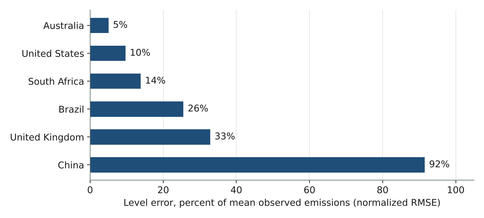
2.Source/make_figures.py.
Where CPAT misses, prices are usually the reason. CPAT computes emissions from fuel use and fuel use from prices, so a projected price that is too low gives too much fuel use and too many emissions. China is the clear case: projected domestic prices ran below observed prices, and the back-cast overstated emissions (Campmas et al. 2023). On coal used for power across all countries, the documentation contradicts itself: its text says CPAT’s projected prices were “on average, above observed prices”, while the same sentence describes the ratio of projected to observed prices as concentrated “under the value of 1”, that is, below. The China case fits the second reading. Observed domestic prices were also often smoother than projected ones, consistent with price regulation that the back-cast did not model. The United Kingdom does not fit the price explanation: the model projected lower emissions despite lower modeled prices, and modeling the UK’s mid-2010s policies would widen the gap. The documentation leaves the UK result unexplained.
The back-cast shows what a no-policy elasticity model can and cannot do. It captures the trend of emissions in most of the six countries. It does not reproduce year-to-year volatility, and for some countries it is persistently above or below history. Two of the three explanations the documentation offers, policies not modeled and price forecasting, are limits of a baseline run rather than faults in the method. The third, a single set of elasticities with no distinction between short and long run, is a fault: the documentation suggests that separate short- and long-run elasticities would track history better (Campmas et al. 2023). The record of long-run energy forecasting gives a reason to be careful with good fits too: US energy projections that were close in total were close because large errors in their components offset (O’Neill and Desai 2005), and a back-cast with observed world prices removes the hardest component.
Six countries are too few, and none is a typical CPAT client. The six are large emitters with good data; most countries that use CPAT are low- and middle-income economies with thinner data and more regulated prices. The back-cast says little about how CPAT performs for them. Historical simulations are rare for integrated models generally, and cannot show that a model will be reliable outside the range of past experience (Wilson et al. 2021), which is where a carbon price of $75 lies for most of these countries.
6 Comparisons with other models and with history
6.1 Price response: the same slope as Enerdata
CPAT’s response of emissions to a carbon price has about the same slope as Enerdata’s. The documentation runs carbon prices of $0 to $120 per tonne of CO₂ in 2030 through both CPAT power models and compares the resulting world emissions in 2030, indexed to each model’s own baseline, with Enerdata’s marginal abatement cost curves. For total CO₂, power-sector CO₂ and greenhouse gases excluding land use, it finds “good alignment” for both of CPAT’s power models (Campmas et al. 2023). Indexing to each baseline removes baseline differences, so this is a clean test of the response. A second comparison, against Enerdata’s Enerbase scenarios for 2025, 2030 and 2035, finds “similar slopes” and, for power-sector CO₂, that CPAT’s simpler “average” power model comes closer to Enerdata than its engineering power model.
6.2 Ex-post evidence: inside a wide range
CPAT’s response to a $10 carbon price is of the same order as the best cross-country estimate. The documentation ran a $10/tCO₂ step for 171 countries over 2019–2035 and computed “semi-elasticities”: the average percentage gap between CO₂ in the policy run and in the baseline, over the first five years (short term) and over the whole period (long term). Table 3 reports them.
| Sector | Short term (2019–2023) | Long term (2019–2035) |
|---|---|---|
| All sectors | −2.4 | −6.2 |
| Industry | −2.7 | −6.2 |
| Power | −2.3 | −8.4 |
| Residential | −2.2 | −4.9 |
| Transport | −0.9 | −2.0 |
Source: Campmas et al. (2023), section “How does CPAT compare to the literature?”, table “Short- and long-term semi-elasticities of CO2 emission in CPAT”. Notes: 171 countries; the short term is the average of the annual gaps over 2019–2023, the long term over 2019–2035.
The documentation’s comparison with the ex-post literature sets two different measures side by side. It finds CPAT “comparable” with a literature whose estimates are “minimal to modest”, 0 to 2 percent a year (Green 2021; Campmas et al. 2023). But CPAT’s figures are average level gaps, while the ex-post studies mostly estimate an annual effect, often on the growth rate of emissions, under whatever price and coverage each scheme had. On a common basis, if a $10 price slows the growth of emissions by g a year, the level gap after k years is about gk, and its average over the first N years is g(N+1)/2. CPAT’s −2.4 percent over five years then corresponds to g ≈ 0.8 percent a year, and its −6.2 percent over 17 years to g ≈ 0.7 percent a year (author’s calculation; the linear build-up is an assumption, and it overstates g for the part of CPAT’s response that is immediate). Rafaty et al. (2020), the cross-country study most like CPAT’s exercise, estimate that each dollar of carbon price slows emissions growth by 0.05 percent a year, or about 0.5 percent a year at $10, an estimate they call imprecise. CPAT is therefore of the same order as the best per-dollar estimate, and somewhat larger.
The rest of the ex-post literature is too wide to say whether CPAT over- or under-responds. Green’s review of 37 studies finds aggregate reductions of 0 to 2 percent a year (Green 2021). A later systematic review and meta-analysis of 80 causal evaluations of 21 schemes finds statistically significant total reductions of 5 to 21 percent (4 to 15 percent after correcting for publication bias), “despite the low level of prices in most instances” (Döbbeling-Hildebrandt et al. 2024). Across 142 countries, emissions from fuel combustion grew about 2 percentage points a year more slowly where a carbon price existed (Best et al. 2020). These figures are for real schemes with low coverage, generous free allocation or both, and they do not scale simply to a comprehensive $10 price; the meta-analysis names the price elasticity of emissions as an evidence gap. The ex-post evidence therefore bounds CPAT loosely rather than testing it.
The sector pattern agrees with the evidence. The power sector shows the largest long-run response in CPAT, as it does in Rafaty et al. (2020), who find most abatement in electricity and heat, and transport the smallest. This is the firmest finding of the comparison, because it does not depend on matching metrics.
6.3 Power: the same mix as the World Bank’s planning model, smoother investment
CPAT’s engineering power model gives a generation mix close to EPM’s in most countries compared. EPM is the World Bank’s least-cost capacity expansion and dispatch model, with hourly renewable availability, ramping limits, reserves, storage and transmission constraints (Campmas et al. 2023). The comparison set CPAT’s 2030 carbon price at about $40/tCO₂ by goal seek, to approximate EPM’s carbon budgets, which are mostly 40 percent below business as usual, and compared electricity demand, generation by fuel and new investment for 14 countries in the main text (Egypt, Iraq, Jordan, South Africa, Türkiye, Ukraine, Vietnam and seven in Africa) and 20 more, all in Africa, in Appendix H. The documentation finds similar fuel types and shares in the mix, with EPM showing more wind in some countries such as Vietnam.
The models differ most on the timing of investment, and the comparison is approximate by design. EPM, as an optimization model, builds in lumps; CPAT spreads new investment over time. For developing countries, where EPM often suggests discontinuous generation and investment, the documentation finds parallels hard to draw (Campmas et al. 2023). The policies are matched only approximately (EPM’s budget looks to 2040, CPAT’s goal seek to 2030), fuel categories are mapped by hand, and storage is not compared. CPAT is therefore supported as a source of plausible mixes, not of investment schedules; a ministry needing an investment plan should use a planning model.
6.4 Air pollution: conservative against global datasets
CPAT’s air-pollution module tends to understate the share of fine particles that comes from fossil fuels. The documentation compares CPAT’s ambient PM2.5 death rates with the Global Burden of Disease 2019 estimates (GBD 2019 Risk Factors Collaborators 2020), its PM2.5 emissions from transport and power with EDGAR and IIASA inventories, and its fossil-fuel share of ambient PM2.5 with the GEOS-Chem estimates of Vohra et al. (2021; CPAT Team 2023). Depending on which of CPAT’s methods links emissions to concentrations, Vohra and coauthors’ fossil share is higher than CPAT’s in 61 percent of countries (averaged intake fraction and FASST local study), 55 percent (machine learning) or 44 percent (FASST local study alone). The chapter concludes that its default configuration gives a conservative fossil contribution, so CPAT is likely to understate the health benefits of a climate policy. It adds that good agreement on baselines does not guarantee agreement on policy impacts, which need checking country by country.
7 Sensitivity: the price elasticities dominate
Of all the parameters tested, the price elasticities move CPAT’s results most. The documentation runs the G20 countries with a carbon tax rising from $10 to $75 in 2030 and changes one parameter at a time. With default settings, CO₂ falls 29 percent against the baseline in 2030. Table 4 and Figure 2 show how that cut changes (Campmas et al. 2023).
| Parameter changed | Setting | CO₂ cut in 2030 | Change (pp) |
|---|---|---|---|
| Default settings | −29% | ||
| Price elasticities | +2 standard deviations | −39% | +10 |
| +1 standard deviation | −35% | +6 | |
| −1 standard deviation | −20% | −9 | |
| −2 standard deviations | −7% | −22 | |
| Power model | Elasticity model | −34% | +5 |
| Engineering model | −22% | −7 | |
| International energy prices | +50% | −20% | −9 |
| −50% | −31% | +2 | |
| EIA forecast | −32% | +3 | |
| Renewables growth limit | Very high | −32% | +3 |
| Income elasticities | ±1 or ±2 standard deviations | −29% | 0 |
| Fiscal multipliers | ±1 standard deviation | −29% | 0 |
| GDP growth | ±50% | −29% to −30% | 0 to +1 |
| Logit parameter k (power) | 6 or 10 | −29% | 0 |
Source: Campmas et al. (2023), section Parameter Sensitivity Analysis, table “CPAT’s parameters sensitivity results”. Notes: G20 countries; one parameter changed at a time. “Change” is the difference between the percentage cut and the default cut, in percentage points; positive means a larger cut. The default power model is the average of the elasticity and engineering models. Rows with negligible effects for other settings are omitted. The documentation does not say how the standard deviations of the elasticities are defined.
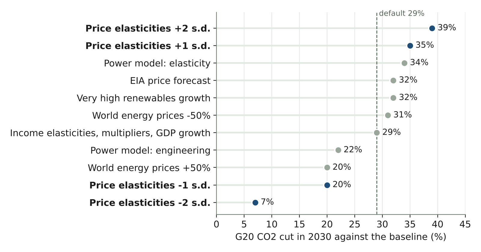
2.Source/make_figures.py.
Three lessons follow. First, the price elasticities deserve the most validation effort: a two-standard-deviation error shifts the 2030 cut by up to 22 percentage points, and the effect is asymmetric, larger for lower elasticities. Second, the choice of power model matters about as much as a one-standard-deviation error in the elasticities, so a ministry should be told which model a result uses. Third, the international price path matters asymmetrically: high world prices leave less for a carbon tax to do, because the tax is a smaller share of the final price. Income elasticities, fiscal multipliers and GDP growth barely affect the percentage cut, although they matter for the baseline level and for GDP results, which this analysis does not test. The design changes one parameter at a time, so it misses interactions, for example high elasticities combined with the engineering power model.
The panel evidence finds most of CPAT’s elasticities in the right range, with clear exceptions in residential electricity and services. The documentation’s panel estimates for 2000–2018 (between, pooled and common-correlated-effects estimators, the last following Pesaran (2006)) find CPAT’s elasticities “in the same ballpark” for most fuels and sectors (Campmas et al. 2023). Residential electricity has an estimated price elasticity of −0.1 against CPAT’s −0.4, and an income elasticity of 0.16 against 0.65. Industrial natural gas has income elasticities of 0.33–0.56 against CPAT’s 0.81. Services fuels respond much like residential ones in the estimates, where CPAT assumes they respond more strongly than industry; the documentation flags this as the main gap to explore. The estimated time trends differ in sign from CPAT’s autonomous efficiency improvements for several fuels.
For gasoline, the panel estimate is lower than the wider literature, so CPAT’s value is uncertain rather than too high. The panel estimate of the price elasticity of gasoline in transport is −0.19 against CPAT’s −0.61, but it comes from the one estimator that passed the documentation’s tests, an estimator whose ability to capture long-run effects in a static model the documentation calls “not clear” (Campmas et al. 2023). A meta-analysis of gasoline demand finds mean price elasticities of −0.34 in the short run and −0.84 in the long run (Brons et al. 2008). CPAT’s −0.61 lies between them. Paper 5.4 takes up this evidence in full (Stretton 2026b); together with Table 4, it suggests that the clearest risk of overstated response is in residential electricity and services, and that the transport elasticity needs a decision between short- and long-run values rather than a cut.
8 Replication across implementations: independent code reproduces legacy CPAT
The CPAT-AI rebuild tested whether the method can be reproduced, block by block, by independent code. Each block of legacy CPAT was reimplemented in Python, fed legacy’s own cached inputs with legacy’s bugs switched back on, and required to reproduce legacy’s stored results. The rebuilt Excel workbook (Excel-AI) was then checked against the Python references with the bugs fixed, and the Python model (Coded CPAT) against Excel-AI (CPAT-AI project 2026b, 2026a; Stretton 2026c). Table 5 summarizes the published results.
| Comparison | What is reproduced | Largest relative difference |
|---|---|---|
| Python reference = legacy: road engineer model | 1,091 series per run, 2022–2041, baseline and carbon tax | 3.8 × 10⁻¹⁴ |
| Python reference = legacy: power prices and costs | 80 legacy rows | 5.6 × 10⁻¹⁷ |
| Python reference = legacy: power engineer model | 208 legacy rows of the baseline and a carbon-tax run | Within 10−13 |
| Python reference = legacy: distribution | Effects, recycling, net effect, compensation; Gini changes | 4 × 10⁻⁴; 7 × 10⁻⁶ |
| Excel-AI = Python reference: power, transport | Every power row in every test scenario; road model in scenarios 1–2 and five copied scenarios | About 5 × 10⁻¹⁵; 5 × 10⁻¹⁴ |
| Coded CPAT = Excel-AI: mitigation | 7,458 output codes per scenario, Egypt, scenarios 1–2, 2022–2041 | Within 10−9 (test tolerance) |
| Coded CPAT = Excel-AI: distribution | 1,684 codes, basket and deciles | Within 10−9 (test tolerance) |
Source: CPAT-AI project (2026b) (check sections of the power, road transport and distribution chapters); CPAT-AI project (2026a). Notes: Each source defines its own relative difference: the road check divides by max(10−6, |legacy|); Coded CPAT’s tests use a relative tolerance of 10−9 (absolute near zero). The distribution figures are limited by the precision of legacy’s cache. Legacy is CPAT 1.0pre_456.
Replication with the bugs fixed shows how far legacy’s results moved. Coded CPAT, which equals Excel-AI, was compared with legacy’s cached Egypt baseline on 272 rows. In the base year 2022, 81 percent of energy-use rows agree within 1 percent and 91 percent within 5 percent; all 15 CO₂ rows agree within 5 percent, with a median gap of 1.2 percent. After the base year, energy use still agrees within 1 percent for about 80 percent of rows, but the CO₂ and price gaps widen: in 2030 the median CO₂ gap is 12 percent and only 12 percent of after-tax price rows agree within 5 percent (CPAT-AI project 2026a). The comparison report attributes the price gaps to a newer data vintage (prices through 2024 rather than 2022) and to fixed legacy price bugs, and the energy and CO₂ gaps to those prices and to fixed fuel-use and emission-factor bugs. The rebuild agrees with legacy where both use the same data and diverges where it corrects legacy, which is what a faithful rebuild should do.
Replication matters for validation because the published validation was run on legacy versions with bugs. The rebuild’s register lists 231 legacy bugs at release 1.1.0 (228 at release 1.0.2), 24 of them of high priority, including a population path for Egypt that departed from the United Nations projection of 147 million people in 2041 (United Nations, Department of Economic and Social Affairs, Population Division 2024), an income factor on the GDP elasticity of power demand applied twice, and services electricity demand growing with industry (CPAT-AI project 2026d; Stretton 2026c). The register does not record which of these were present in the versions used for the back-cast (1.0pre_043) or the model comparisons, whose version the documentation does not state. But several affect exactly the baseline paths those exercises tested. The published validation is therefore evidence about an earlier model, not about the corrected one.
The public rebuild limits what outsiders can rerun. Six of CPAT’s data tables are proprietary (energy balances, energy consumption, domestic prices, input-output tables, the household survey and transport data). The public repository holds them only for Egypt, perturbed within 3 percent, so an outside reader can reproduce the method but not the country results (CPAT-AI project 2026c).
9 Where CPAT fits well and where it does not
CPAT fits well where its structure matches the question. Base-year energy use and emissions are right by calibration. Back-cast emission levels for large economies with market-based prices are within 5 to 14 percent of mean emissions (Australia, the United States, South Africa). The response of emissions to a carbon price has the same slope as a detailed global energy model, is of the same order as the best cross-country ex-post estimate, and ranks sectors as the ex-post evidence does (power most, transport least). The power mix under a moderate carbon price is close to that of a full planning model. And the method can be reproduced exactly by independent code, so its results are not artifacts of a particular workbook.
CPAT fits poorly where prices are regulated, data are thin or responses take time. Back-cast errors are large for China and sizable for Brazil and the United Kingdom, mostly because modeled domestic prices diverged from observed ones. Year-to-year volatility is not reproduced. Investment timing in power differs from an optimization model. The elasticities for residential electricity and services look high against panel estimates, and the transport elasticity mixes short- and long-run evidence. Calibration can carry a data break, such as Egypt’s inventory jump in 2022, into every projected year.
Road transport is described three times in CPAT, and no published check tests the three against each other. CPAT models road transport in a simple fuel equation, in an engineering fleet model and in a co-benefits module that values congestion, accidents and road damage. The three are not consistent: the co-benefits module always takes vehicle-kilometers from the fleet model, even when fuel use and emissions follow the fuel equation, so the change in driving it values need not match the modeled change in fuel use (CPAT-AI project 2026d, no. I100; Stretton 2026a).
For a ministry, the practical reading is to use CPAT for ranges and comparisons, not point forecasts. A CPAT estimate that a carbon tax cuts emissions by 29 percent should be read as “between about 20 and 35 percent, depending mainly on the elasticities and the power model”, the range that one standard deviation in the elasticities and the choice of power model give in Table 4 (author’s reading; the documentation attaches no probability to it). Comparisons across policies run on the same baseline are more reliable than levels, because baseline errors largely cancel. Where a result hinges on residential electricity, services or road fuels, the elasticities should be checked against national evidence.
10 What validation remains
Rerun the published validation on the corrected model, for every country. Coded CPAT runs one country and two scenarios in under a second (CPAT-AI project 2026a), so the back-casts, model comparisons and sensitivity runs can be repeated for every country with data, as automated tests rather than one-off studies. This requires the full CPAT database, whose six proprietary tables the public rebuild holds only for Egypt, perturbed.
Report a measure of fit for every comparison. The baseline, price-response and power comparisons are published as charts. A renewed validation should report, for each country and indicator, the error against each reference (mean absolute percentage error or normalized RMSE), so that users can see where the model is close and where it is not, and so that each new version can be checked against the last.
Make the back-cast a true forecast test. The published back-cast fed in observed world prices, which removes the hardest part of forecasting. A full back-cast would also use the international price forecasts available at the base year, and would include each country’s price regulations and major policies. It should cover low- and middle-income countries, not only large emitters, and report errors by component (activity, energy intensity, carbon intensity) as well as in total, since totals can be right for the wrong reasons (O’Neill and Desai 2005; Koomey et al. 2003).
Validate policy responses against natural experiments, on a common metric. The strongest test of a carbon-pricing model is whether it predicts the effect of carbon prices that were actually introduced, such as Sweden’s or British Columbia’s, given the data available before they started. The ex-post literature now offers enough cases to do this country by country (Green 2021; Döbbeling-Hildebrandt et al. 2024). CPAT should report its response in the same form as the studies it is compared with, as an effect on the growth rate per dollar of carbon price, rather than as an average level gap.
Settle the elasticities. Table 4 shows that no other parameter matters as much. Paper 5.4 compares CPAT’s elasticities with the panel evidence and published meta-analyses (Stretton 2026b); the demand system that links them to the Total Effective Carbon Price is in paper 6.1 (Stretton 2026d). Separate short- and long-run elasticities, which the documentation recommends, would also address the back-cast’s volatility problem.
Fix the documentation’s own errors. Three are found here: the coal-price table in the back-cast section repeats the energy CO₂ table; the same section states the direction of the coal-price error both ways; and the CPAT-AI documentation’s “16–29 percent” understates Egypt’s calibration gap in 2023. The rebuild has registered and corrected 20 other documentation errors (CPAT-AI project 2026d). A validation that readers cannot reproduce from its documentation is weaker than it needs to be.
11 Conclusion
CPAT’s published validation, read as a whole, supports its use for first estimates of the direction and size of carbon pricing’s effects and for comparisons across policies. It does not support reading its outputs as point forecasts, especially where prices are regulated or data are thin. Two conclusions change on a closer reading of the evidence: CPAT’s response to a carbon price is not shown to be too large, because the ex-post literature is too wide and uses a different metric; and its gasoline elasticity is uncertain rather than too high, while residential electricity and services are the clearer gaps. What is new here is the assembly, the recomputation and the corrections: the documented tests set side by side, their numbers in tables, three source errors found, and the replication evidence from the rebuild added. The main limitation is that every published check predates the correction of more than 200 legacy bugs, so the evidence is about an earlier model. The next step is to make validation part of the model’s test suite: rerun the back-casts, comparisons and sensitivity analysis on Coded CPAT for every country, report a measure of fit for each, and repeat them at every release.
Downloads
References
Appendix A. Which numbers are the documentation’s and which are new
| Number in this paper | Status | Source or calculation |
|---|---|---|
| Back-cast RMSE and normalized RMSE (Table 2, Figure 1) | Documentation’s, rounded | Campmas et al. (2023), Hindcasting |
| Implied mean observed emissions (about 9.9 Gt for China, 7.0 Gt for the United States) | Recomputed | RMSE divided by normalized RMSE |
| Semi-elasticities (Table 3) | Documentation’s | Campmas et al. (2023), Ex-post studies |
| Growth-rate equivalents of CPAT’s response (0.8 and 0.7 percent a year) | Author’s calculation | Average level gap = g(N+1)/2 for N = 5 and 17, assuming a linear build-up |
| Rafaty et al.’s response at $10 (0.5 percent a year) | Author’s calculation | 0.05 percent per $1 (Rafaty et al. 2020) times 10 |
| Sensitivity results (Table 4, Figure 2) | Documentation’s | Campmas et al. (2023), Parameter sensitivity |
| “Between about 20 and 35 percent” | Author’s reading | ±1 standard deviation in the elasticities; elasticity or engineering power model |
| Panel elasticities | Documentation’s | Campmas et al. (2023), Panel estimation |
| EPM set-up and country counts (14 + 20; 29 of 34 in Africa) | Documentation’s; counts by the author | Campmas et al. (2023), Model comparisons and Appendix H |
| Air-pollution shares (61, 55, 44 percent) | Documentation’s | CPAT Team (2023) |
| Egypt calibration factor (0.930) and inventory values | CPAT-AI documentation’s | CPAT-AI project (2026b), Emissions |
| Egypt jump (19.5 percent) and gaps (16, 32, 29 percent) | Recomputed | From the CPAT-AI documentation’s table |
| Replication tolerances (Table 5) and legacy comparison shares | CPAT-AI documentation’s | CPAT-AI project (2026b); CPAT-AI project (2026a) |
| Bug counts (231 at release 1.1.0; 228 at 1.0.2; 24 high priority) | CPAT-AI register’s | CPAT-AI project (2026d) |
Footnotes
The validation exercises reported here were carried out by the CPAT team and published in the CPAT methodology (2023 edition, corrected online in October 2026). Its mitigation chapter, including the validation section, was prepared by Alexandra Campmas, Daniel Bastidas, Olivier Lelouch, Faustyna Gawryluk, Paolo Agnolucci and the author; the panel estimation of energy demand is Paolo Agnolucci’s (Campmas et al. 2023). CPAT’s air-pollution module, whose validation Section 6.4 reports, is the work of Paulina Schulz-Antipa (CPAT Team 2023). The replication results come from the CPAT-AI repository, release 1.1.0 (CPAT-AI project 2026c). This paper selects, condenses, recomputes and interprets; Appendix A lists which numbers are the documentation’s and which are new. Errors of interpretation are the author’s own.↩︎