Measure Carbon Pricing by the Emissions It Cuts
The Total Effective Carbon Price
Countries cut emissions with taxes, subsidies, standards and mandates, but the standard metrics add up explicit prices per tonne. They score a fuel standard or a revenue-neutral feebate at zero and count a dollar on coal the same as a dollar on gasoline. Building on the IMF’s carbon-price equivalent, this paper derives the Total Effective Carbon Price: the uniform economy-wide carbon tax that would cut emissions by as much as a given policy mix. From a nested constant-elasticity model of energy demand I obtain closed-form abatement weights that split any instrument’s effect into fuel switching and demand reduction. I give exact and second-order versions and a version for any horizon, extend the metric to tradable and non-tradable standards and mandates, and carry elasticity uncertainty through to a range. In a stylized three-sector economy, a mix that explicit-price metrics rate at $21 per tonne has an effective price of $37 in the long run ($32–38 across calibrations) and $28 after one year. The metric lets crediting schemes pay for policies rather than projects, lets border mechanisms recognize implicit and non-price carbon pricing, and shows governments where their policy mix is weak.
carbon pricing, effective carbon price, carbon price equivalent, non-price instruments, energy demand, policy crediting
Working paper, version 0.4, October 2026. Stephen J. Stretton, writing in a personal capacity. The views expressed are the author’s own and do not represent those of any institution with which he is or has been affiliated. A short version for policy makers is Climate Fiscal Policy Brief No. 6.1. Version 0.2 (May 2026) and earlier versions carried an error in the fuel-switching elasticity; Appendix E sets out the correction.
Keywords: carbon pricing; effective carbon price; carbon price equivalent; non-price instruments; energy demand; policy crediting. JEL: H23, Q41, Q48, Q54, Q58, C43.
1 Executive summary
Policy brief (short version) → · Download this paper (pdf) · Slides (pdf)
Headline carbon prices misstate how hard countries push on emissions. Governments cut emissions with carbon taxes and emissions trading, but also with fuel taxes, subsidies for clean power, fuel standards, efficiency rules and procurement mandates. The measures used to compare countries, such as the OECD’s effective carbon rate and the World Bank’s total carbon price, add up explicit prices per tonne of CO₂, weighted by emissions: the price signal, not what it achieves. A fuel standard scores nothing, a feebate that charges dirty producers and rebates clean ones scores nothing because its average payment is zero, and a dollar per tonne on coal counts the same as a dollar on gasoline, although it cuts far more.
This paper measures a policy mix by the emissions it cuts. The Total Effective Carbon Price (TECP) is the single, economy-wide carbon tax that would cut emissions by as much as the actual mix, against the same baseline and over the same horizon. A tax of $30 per tonne on every fuel is worth exactly $30. The idea of such a carbon-price equivalent is not new: the IMF computes it with its Climate Policy Assessment Tool, one model run per policy. What this paper adds is a way to compute it from a country’s energy balance, fuel prices and two published elasticities per sector, without a model run, and to see where each dollar of it comes from.
The calculation splits every policy into two effects: switching to cleaner fuels and using less energy. A carbon tax does both. A feebate works almost only through switching. A tax per unit of energy works only through demand. A renewable subsidy works through switching but loses a little through demand, because cheaper power raises consumption. Weights computed once per country turn any package into one number, and that number splits by sector, by instrument and by effect. A short correction makes the closed form accurate to within 2 percent in the worked example; a full model gives the exact value.
Standards and mandates fit on the same scale. A tradable standard behaves like a feebate at its credit price, so it enters the same formula. A standard that cannot be traded enters at the average marginal cost of compliance, weighted by how strongly each firm responds. A mandate or a procurement rule enters through its measured effect on emissions, under stated conditions.
In a stylized three-sector economy, explicit prices rate a policy mix at $21 per tonne; the TECP rates it at $37 in the long run and $28 after one year. The mix is a $30 carbon tax on power and industry, a $10 per megawatt-hour subsidy to renewable power and a fuel standard that cuts the carbon intensity of road fuel by 2 percent. The tax alone is worth $27, because it falls on the sectors where emissions respond most. The fuel standard has a credit price of $166 per tonne but adds only $1, because road fuel responds little at the margin. Across the published range of elasticities, the long-run TECP lies between $32 and $38 in 90 percent of draws and always exceeds the explicit price. The central case sits toward the top of that range because its demand elasticities are low; with the demand elasticities of the IMF-World Bank model it is $33.
The metric has three uses. First, climate-finance facilities can pay for policies rather than projects: a country that adopts a fuel standard or a feebate earns the same per tonne as one that taxes. Second, border mechanisms such as the EU’s Carbon Border Adjustment Mechanism can credit the carbon price signal of feebates and standards, which today earn nothing because they pay nothing net. Third, governments can see where their package is weak: in the example, extending the carbon tax to road fuel would add only $1.6 to the TECP.
The TECP measures abatement, not cost. Two packages with the same TECP cut the same tonnes but need not cost the same; standards and subsidies usually cost more per tonne than a price. The TECP should be reported beside each instrument’s shadow price and cost. The main next step is to compute it for a real country from its energy balance and to compare it with the IMF’s model-based equivalent for the same policies.
2 Introduction
Headline carbon prices misstate how hard countries are pushing on emissions. No country prices carbon with one instrument. A typical package combines a carbon tax or emissions trading in power and industry, fuel excises, renewable subsidies, a clean-fuel standard and efficiency rules. The metrics used to compare countries, the OECD’s effective carbon rate and the World Bank’s total carbon price, add up explicit and indirect prices per tonne of CO₂ and weight them by emissions (OECD 2023; Agnolucci et al. 2024). They measure the price signal, not what it achieves. A clean-fuel standard or a renewable subsidy scores nothing, a revenue-neutral feebate scores nothing because its average payment is zero, and a dollar per tonne on coal counts the same as a dollar on gasoline although it cuts far more. The authors of the World Bank measure say so: it describes the incentive, not the mitigation, and an effectiveness-weighted version is future work (Agnolucci et al. 2024, sec. 6.4).
The question this paper answers is what single carbon tax a package of instruments is worth. The Total Effective Carbon Price (TECP) is the uniform economy-wide carbon tax that would cut emissions by as much as the actual policy mix, against the same baseline and over the same horizon. A tax at $X per tonne on every fuel returns exactly $X. Any other instrument, price-based or not, is scored by its emission effect in units of that tax.
The concept is not new; a computable, decomposable version is. Weil (2021) defines a jurisdiction’s carbon price equivalent as the carbon price that, in an otherwise neutral policy environment, would produce the same emissions as its actual policy mix, and proposes it for comparing effort and for border adjustments. The IMF computes economy-wide and sectoral carbon price equivalents for the G20 by re-simulating its Climate Policy Assessment Tool (CPAT) (Black et al. 2022), and its proposal for an international carbon price floor would weight fuel taxes by their relative effectiveness at cutting economy-wide emissions (Parry, Black, and Roaf 2021). Carhart et al. (2022) go the other way: their comprehensive carbon price adds the marginal incentives of seven instruments, standards and feed-in tariffs included, weighted by the emissions each covers, and leaves the emission effect to future work. The IMF’s equivalents need a model run for each policy; the comprehensive price does not weight by responsiveness. This paper derives the metric in closed form from a nested constant-elasticity-of-substitution (CES) model of energy demand. Abatement weights, computed once per country from the energy balance, delivered prices and two elasticities per sector, convert any package into one number by a weighted sum, and the number splits by sector, by instrument and by margin: fuel switching versus using less energy.
The paper makes five contributions.
- A closed-form first-order TECP (Section 5). Proposition 1 derives the semi-elasticities from the CES cost function: the switching semi-elasticity is \(\sigma_s(e_f/p_{fs} - \kappa_s)\) and the demand semi-elasticity \(\eta_s\kappa_s\), where \(\kappa_s\) is the sector’s emissions per dollar of energy spending. The abatement weight of a sector is its energy spending times \(\sigma_s V_s + \eta_s\kappa_s^2\), where \(V_s\) is the variance of carbon per dollar across its fuels. Proposition 2 shows that the switching margin moves along the isoquant, so it conserves energy service, as it must; earlier versions of this paper did not satisfy that condition (Appendix E).
- Accuracy beyond first order (Section 6). The exact TECP is unique (Proposition 3), and a closed-form second-order correction recovers most of the gap between the linear and the full-model value: in the worked example the first-order TECP is 10 percent low, the second-order 1.7 percent.
- Non-price instruments (Section 7). A tradable standard is a feebate at its credit price (Proposition 4). A non-tradable standard with heterogeneous compliance costs is scored by a responsiveness-weighted average of marginal compliance costs, which reduces to the emission-weighted average when firms respond alike (Proposition 5). Mandates, procurement rules and legal obligations are scored by backing out the price from a modeled emission effect, under stated identification assumptions.
- Timing, calibration and uncertainty (Section 5, Section 8). Because fuel switching needs new capital and demand does not, the TECP has a horizon: the example’s mix is worth $28 after one year and $37 in the long run. Elasticities come from meta-analyses, each cited only for what it estimates, and the uncertainty is carried through to a band by Monte Carlo. Errors common to all elasticities largely cancel; errors in demand elasticities alone do not.
- Comparison (Section 3, Section 9). One stylized economy is scored by the explicit-price metrics, an average-cost implicit price, the comprehensive carbon price, the IMF’s equivalence approach and the TECP. The explicit-price metric says $21; the TECP says $33 to first order and $37 exactly; the comprehensive carbon price, which counts the fuel standard’s credit price on the emissions it covers, says $72.
The metric serves the series it belongs to. Paper 1.1 proposes paying countries per tonne cut by a policy rather than by a project, which needs a common unit for taxes, feebates and standards (Stretton 2026d). Paper 1.4 proposes that the EU’s border mechanism recognize a sector’s price signal rather than only the price paid, which needs a measure of that signal for non-price instruments (Stretton 2026b). Section 10 sets out both uses and a third, country diagnostics. Section 11 states what the metric does not measure.
3 Related literature and existing metrics
Four families of metrics put climate policies on one scale, and only one measures emission effects. Appendix A reviews the literature in full; Table 1 summarizes the comparison and scores the worked example of Section 9 under each.
Price-signal metrics add explicit and indirect prices and weight them by emissions. The OECD’s effective carbon rate sums carbon taxes, emissions trading prices and fuel excise taxes per tonne of CO₂ for each fuel and sector, and its net version deducts fossil-fuel subsidies (OECD 2023). The World Bank’s total carbon price adds direct pricing to indirect pricing through excises and consumption subsidies, measured by a price-gap method, for 142 countries from 1991 to 2021, so it can turn negative; indirect pricing is most of the global total (Agnolucci et al. 2024). Both share the TECP’s cell structure, fuel by sector, which makes the TECP easy to explain: it keeps the cells’ prices and replaces emission weights with abatement weights. Neither counts standards, mandates or subsidies to clean energy. The World Carbon Pricing Database documents explicit instruments by sector (Dolphin and Xiahou 2022). An econometric estimate on a large cross-country panel finds that a €10 rise in the effective carbon rate cuts fossil CO₂ by 3.7 percent in the long run (D’Arcangelo et al. 2022), a semi-elasticity of the same order as the 0.6 percent per dollar in this paper’s example.
The IMF measures gaps to efficient prices, which is a different object. Its subsidy estimates compare retail fuel prices with an efficient price that includes supply costs, environmental costs and forgone consumption taxes; explicit subsidies are undercharging for supply costs and implicit subsidies are undercharging for the rest (Parry, Black, and Vernon 2021; Black, Liu, et al. 2023). A large implicit subsidy means prices are far from efficient. It does not say how much current policy cuts emissions, and only the explicit part is a policy price that could enter the TECP’s cells.
Implicit carbon prices have meant average cost per tonne. The OECD’s 2013 effective carbon prices divide the cost of each policy by the tonnes it abates, across taxes, trading, feed-in tariffs, capital subsidies and regulations (OECD 2013). Marcantonini and Ellerman (2015) compute the implicit carbon price of German feed-in tariffs this way for 2006–2010: tens of euros per tonne for wind and hundreds for solar. J. E. Aldy and Pizer (2016) note that such prices measure average cost, are model-derived and are high both for costly policies and for those that abate little. A metric of this kind ranks an expensive policy as ambitious. The TECP ranks it by what it cuts. “Implicit carbon price” has also meant the shadow cost of a regulation and indirect pricing through fuel taxes (Agnolucci et al. 2024, n. 1).
The comprehensive carbon price counts non-price instruments at their marginal incentive, not their effect. Carhart et al. (2022) measure, for 25 countries that emit 82 percent of global CO₂, the sum over seven instruments (carbon taxes, emissions trading, fossil-fuel taxes and subsidies, renewable portfolio standards, feed-in tariffs and low-carbon fuel standards) of each instrument’s marginal incentive in dollars per tonne times the share of the country’s emissions it covers. They find a global comprehensive carbon price of about $19 per tonne in 2019 and country values from −$128 to +$146, and they name emissions abatement as future research. Their metric is the right one for asking what marginal incentive emitters face; the TECP is the right one for asking what the incentives achieve. In the worked example the two differ by a factor of two.
Carbon price equivalents measure emission effects, and the TECP is one. Weil (2021) states the concept for the whole economy: the carbon price that, applied in an otherwise neutral policy environment, would produce the same emissions as a jurisdiction’s actual policies, or equivalently the allowance price of a cap-and-trade system whose cap matched observed emissions. He proposes it for strategic emissions policy and for border adjustments of domestic taxes and regulations, and discusses the baseline, currency conversion and production against consumption emissions; he does not compute it. Black et al. (2022) define the economy-wide and sectoral carbon price equivalents as the price that yields the same CO₂ cut as a policy, computed by simulating the policy in CPAT and searching for the matching carbon price. For the G20 in 2030 they find sectoral equivalents above $150 per tonne in ten cases for power-sector renewables and coal phase-out targets, and $5–40 per tonne in most cases from existing fuel taxes. CPAT represents non-price policies by shadow prices on the efficiency margin (Black et al. 2022; Black, Parry, et al. 2023), and the IMF supplements it with capital-turnover models for vehicles and buildings. The IMF’s price-floor proposal accepts “emissions-equivalent alternatives to carbon pricing” and proposes weighting fuel taxes by relative effectiveness (Parry, Black, and Roaf 2021), and the 2019 Fiscal Monitor describes effective carbon prices computed by weighting CO₂-equivalent fuel taxes and direct carbon prices by their relative effectiveness (International Monetary Fund 2019, Box 1.2). The exact TECP of Section 6 is the same object as Weil’s and the IMF’s economy-wide equivalent. The differences are in construction and use: a closed-form linear version that needs no model run, weights that belong to the economy and can be published, a split by margin that explains why feebates, standards and portfolio standards deliver less abatement per dollar of shadow price than a tax, an explicit theory of non-price instruments, and an uncertainty band.
2.Source/make_wp_figures.py.
| Metric | What it counts | How it aggregates | Non-price instruments | What it misses | Example mix ($/t) |
|---|---|---|---|---|---|
| Effective carbon rate (OECD) | Carbon taxes, trading prices, fuel excises; net version less fossil-fuel subsidies | Emission-weighted average | Not counted | Responsiveness; standards; clean-energy subsidies | 20.8 |
| Total carbon price (World Bank) | Direct pricing plus excises net of consumption subsidies (price gap) | Emission-weighted average | Not counted | As above | 20.8 |
| Price gap to efficient prices (IMF) | Gap between retail and efficient fuel prices | Dollars of subsidy by fuel | Not counted | Not a policy price; says nothing about emission effects | n.a. |
| Average-cost implicit price (OECD 2013 type) | Cost of a policy per tonne abated | Per instrument | Counted at average cost | Marginal effect; ranks costly policies high | 78.5 (subsidy) |
| Comprehensive carbon price (Carhart et al.) | Explicit prices, fuel taxes and subsidies, plus credit prices of standards and feed-in tariffs | Covered-emission-weighted | Counted at marginal incentive | Size and responsiveness of the base | 71.8 |
| Carbon price equivalent (Weil; IMF) | Uniform price with the same emission cut, by model re-simulation | Model | Shadow prices in CPAT | Needs a model run per policy; no closed-form weights | 36.9 |
| TECP (this paper) | Uniform tax with the same emission cut | Abatement-weighted average of price wedges; exact by iteration | Credit price, weighted compliance cost or backed-out effect | Cost and welfare; leakage outside the model | 33.2 (first order); 36.9 (exact); 32.4–38.1 (range) |
The emission-effect literature on individual instruments supplies the decomposition’s logic. Fischer and Newell (2008) decompose each power-sector instrument into implicit taxes and subsidies by technology and rank them by cost for a given cut: an emissions price, then a performance standard, a fossil output tax, a renewable portfolio standard, a renewable subsidy and research subsidies. A portfolio standard is a small tax on fossil output and a larger subsidy to renewables, with no conservation incentive. Holland et al. (2009) show that a low-carbon fuel standard taxes high-carbon fuel and subsidizes low-carbon fuel and cannot be first best. A clean energy standard is likewise an implicit tax on dirty and subsidy to clean generation, so it raises electricity prices less than emissions pricing; Goulder et al. (2016) show that this makes it a smaller implicit tax on factors of production and can make it cheaper than emissions pricing for small cuts. In the TECP these are statements about the demand margin: such instruments have small or negative extensive carbon prices, so their TECP lies well below their shadow price.
The model is standard; its use for a policy metric is not. The nested CES goes back to Sato (1967). CPAT, the closest applied model, uses constant-elasticity fuel demands split into a usage margin and an efficiency margin, calibrated to long-run meta-analytic elasticities (Black, Parry, et al. 2023; World Bank and International Monetary Fund 2022). The TECP splits responses into fuel switching and conservation instead, a different axis that maps onto the price wedges instruments create.
4 Energy demand: nested CES with partial adjustment
Each sector minimizes the cost of an energy service produced from several fuels, and buys less service when it costs more. The economy has sectors \(s\) (power, transport, industry, buildings) and fuels \(f\). Sector \(s\) uses \(q_{fs}\) units of fuel \(f\) at delivered price \(p_{fs}\), which includes existing taxes. Fuel \(f\) emits \(e_f\) tonnes of CO₂ per unit, so baseline emissions are \(E_{fs} = e_f q_{fs}\) and \(E_s = \sum_f E_{fs}\). Fuels combine into a service \(Q_s\) through a CES aggregator with elasticity of substitution \(\sigma_s\): \[ Q_s = \Big[\sum_f \alpha_{fs}^{1/\sigma_s}\, q_{fs}^{(\sigma_s-1)/\sigma_s}\Big]^{\sigma_s/(\sigma_s-1)}, \tag{1}\]
with unit cost \(C_s(p) = \big(\sum_f \alpha_{fs}\, p_{fs}^{1-\sigma_s}\big)^{1/(1-\sigma_s)}\). Demand for the service has constant price elasticity \(-\eta_s\), with \(\eta_s \ge 0\) written as a positive number throughout: \(Q_s = \bar Q_s\, (C_s/\bar C_s)^{-\eta_s}\). Cost minimization gives fuel demand \(q_{fs} = Q_s\, \alpha_{fs}\, (p_{fs}/C_s)^{-\sigma_s}\). The share parameters \(\alpha_{fs}\) are calibrated so that the baseline reproduces observed quantities.
Three statistics of the baseline summarize each sector. Energy spending is \(X_s = \sum_f p_{fs} q_{fs}\) and fuel \(f\)’s cost share \(s_{fs} = p_{fs}q_{fs}/X_s\). Carbon per dollar of fuel \(f\) is \(x_{fs} = e_f/p_{fs}\). The sector’s carbon per dollar of energy spending is the cost-share-weighted mean, \[ \kappa_s = \sum_f s_{fs}\, x_{fs} = E_s / X_s , \tag{2}\]
and the dispersion of carbon per dollar across fuels is \(V_s = \sum_f s_{fs}(x_{fs} - \kappa_s)^2\). A sector with one fuel, or with fuels that emit the same per dollar, has \(V_s = 0\): no carbon price can move it by switching. In the worked example, power emits 8.2 kg of CO₂ per dollar of energy spending, industry 7.8 kg and road transport 2.3 kg, because motor fuel is expensive per unit of carbon.
A policy that changes delivered prices moves quantities through a known formula. Let a policy change prices by \(\Delta p_{fs}\), write \(\pi_{fs} = \Delta p_{fs}/p_{fs}\) for the proportional change and \(P_{fs} = 1 + \pi_{fs}\). Relative to the baseline, the CES gives exactly \[ \frac{q'_{fs}}{q_{fs}} = P_{fs}^{-\sigma_s}\,\Big(\frac{C'_s}{C_s}\Big)^{\sigma_s - \eta_s}, \qquad \frac{C'_s}{C_s} = \Big(\sum_f s_{fs}\, P_{fs}^{1-\sigma_s}\Big)^{1/(1-\sigma_s)} . \tag{3}\]
Only observed cost shares and the two elasticities enter: the share parameters drop out. To first order, with \(\bar\pi_s = \sum_f s_{fs}\pi_{fs}\) the change in the sector’s cost index, \[ d\ln q_{fs} = \underbrace{-\sigma_s\,(\pi_{fs} - \bar\pi_s)}_{\text{fuel switching}} \;\underbrace{-\;\eta_s\,\bar\pi_s}_{\text{demand}} . \tag{4}\]
The first term reallocates use among fuels in proportion to how far each fuel’s price moves relative to the sector’s cost index. The second scales all fuels down with the cost index. This is the isoelastic form of the CES: the elasticity of fuel \(f\) with respect to the price of fuel \(g\) is \(\varepsilon_{fg} = -\sigma_s\delta_{fg} + (\sigma_s - \eta_s)s_{gs}\), an \(n \times n\) matrix generated by two parameters and the cost shares, with symmetry and the adding-up conditions built in (Appendix C).
The CES discipline matters because unconstrained elasticities do not add up. An isoelastic model with free own- and cross-price elasticities needs \(n^2\) parameters per sector and, estimated piecemeal, need not satisfy the restrictions that make switching conserve energy service. The cost of the discipline is that one \(\sigma_s\) governs every pair of fuels in a sector. Stern’s meta-analysis finds that in industry substitution is easy between most pairs of fuels, with elasticities between oil and coal, oil and gas, oil and electricity, and gas and electricity significantly above one, and harder at the level of the whole economy (Stern 2012), so a single \(\sigma_s\) is an average over pairs that differ. Where the spread matters, a further nest, gas against coal within fossil fuels and fossil against clean above it, lets the elasticities differ.
Fuel switching needs new capital; using less energy does not, so the two margins adjust at different speeds. Write fuel demand as \(q_{fs} = Q_s\, h_{fs}(p)\), where \(h_{fs}\) is the unit input requirement of fuel \(f\) per unit of service; the switching term of equation 4 moves \(\ln h_{fs}\) and the demand term moves \(\ln Q_s\). Each moves a fixed fraction of the way to its new equilibrium each year: \[ \ln h_{fs,t} = \ln h_{fs,t-1} + \lambda^{I}_s\big(\ln h^{*}_{fs,t} - \ln h_{fs,t-1}\big), \qquad \ln Q_{s,t} = \ln Q_{s,t-1} + \lambda^{X}_s\big(\ln Q^{*}_{s,t} - \ln Q_{s,t-1}\big). \tag{5}\]
After a permanent price change, the switching margin has completed a fraction \(a^I_s(T) = 1 - (1-\lambda^I_s)^T\) of its long-run response by year \(T\), and the demand margin \(a^X_s(T) = 1 - (1-\lambda^X_s)^T\). The horizon-\(T\) elasticities are \(a^I_s(T)\sigma_s\) and \(a^X_s(T)\eta_s\), and with one-year and long-run estimates from the literature, \(\lambda \approx \varepsilon^{SR}/\varepsilon^{LR}\) (Labandeira et al. 2017; Havranek et al. 2012). Switching between fuels in vehicles, boilers and furnaces follows capital turnover, a few percent of the stock a year (Black et al. 2022, Annex C, for vehicles); behavioral demand responds within one or two years. So \(\lambda^I_s\) is small and \(\lambda^X_s\) large. Splitting the adjustment into the two CES components keeps the switching margin on the isoquant at every date (Appendix C).
Technical efficiency changes units, not the TECP. Prices and emission factors can be expressed per unit of useful energy, \(p/\varphi\) and \(e/\varphi\), where \(\varphi\) is conversion efficiency. Carbon per dollar, \(x = e/p\), and cost shares are unchanged by that rescaling, so every result below holds whether quantities are measured in final or useful energy. Efficiency matters only where Proposition 2(ii) refers to equal prices per unit of service.
5 The Total Effective Carbon Price
The TECP is defined by an emission cut, not by a formula. Let \(R(\tau)\) be the full-model emission cut, relative to the baseline and at horizon \(T\), from a carbon tax of \(\tau\) per tonne on every fuel in every sector, so that \(\Delta p_{fs} = \tau e_f\). Let \(R_P\) be the cut from a policy mix \(P\), in the same model, against the same baseline and at the same horizon.
Definition 1 (TECP). The Total Effective Carbon Price of \(P\) is the \(\tau^*\) that solves \(R(\tau^*) = R_P\).
The definition says what the TECP measures: abatement, in units of a uniform tax. Proposition 3 below shows that \(\tau^*\) exists and is unique. Computing it needs the full model; the first-order version needs only weights.
To first order, the TECP is a weighted average of the prices a policy puts on each fuel. Define the policy’s extensive carbon price in sector \(s\) and its intensive carbon price on fuel \(f\) as \[ \tau^{\mathrm{ext}}_s = \frac{\bar\pi_s}{\kappa_s}, \qquad \tau^{\mathrm{int}}_{fs} = \frac{\pi_{fs} - \bar\pi_s}{x_{fs} - \kappa_s}. \tag{6}\]
The extensive price is the uniform carbon tax that would raise the sector’s cost index as much as the policy does. The intensive price is the uniform carbon tax that would move fuel \(f\)’s price relative to the cost index as much as the policy does. Both are in dollars per tonne, and a carbon tax at rate \(\tau\) sets both equal to \(\tau\) for every fuel in every sector it covers. The intensive price is undefined for a fuel whose carbon per dollar equals the sector average, but its product with the semi-elasticity below is always defined.
Proposition 1 (first-order TECP). Let the economy follow the nested CES of equation 1, and let a policy change delivered prices by \(\Delta p_{fs}\). To first order in the price changes:
(i) the emission cut is \[ R_P = \sum_s\Big[\sum_f E_{fs}\,\tilde\varepsilon^{\,\mathrm{int}}_{fs}\,\tau^{\mathrm{int}}_{fs} + E_s\,\tilde\varepsilon^{\,\mathrm{ext}}_s\,\tau^{\mathrm{ext}}_s\Big], \qquad \tilde\varepsilon^{\,\mathrm{int}}_{fs} = \sigma_s\,(x_{fs} - \kappa_s), \quad \tilde\varepsilon^{\,\mathrm{ext}}_s = \eta_s\,\kappa_s ; \tag{7}\]
(ii) a uniform tax of $1 per tonne cuts emissions by \[ \Lambda = \sum_s X_s\big(\sigma_s V_s + \eta_s\kappa_s^2\big) > 0 ; \tag{8}\]
(iii) the first-order TECP is \[ \tau^*_{(1)} = \frac{R_P}{\Lambda} = \sum_s\sum_f \Omega^{\mathrm{int}}_{fs}\,\tau^{\mathrm{int}}_{fs} + \sum_s \Omega^{\mathrm{ext}}_s\,\tau^{\mathrm{ext}}_s, \qquad \Omega^{\mathrm{int}}_{fs} = \frac{E_{fs}\tilde\varepsilon^{\,\mathrm{int}}_{fs}}{\Lambda}, \quad \Omega^{\mathrm{ext}}_s = \frac{E_s\tilde\varepsilon^{\,\mathrm{ext}}_s}{\Lambda}, \tag{9}\]
with weights that sum to one; and (iv) a uniform tax at rate \(\tau\) has \(\tau^*_{(1)} = \tau\).
The proof (Appendix B) differentiates equation 3. The semi-elasticities have direct readings. Switching cuts emissions from fuel \(f\) in proportion to how far its carbon per dollar exceeds the sector’s: a $1 tax raises fuel \(f\)’s price by \(e_f\), or \(x_{fs}\) in proportion, against \(\kappa_s\) for the cost index. Demand cuts all of a sector’s emissions in proportion to its carbon per dollar of energy spending. A sector’s switching weight is \(\sigma_s X_s V_s/\Lambda\): large where clean and dirty fuels coexist at very different carbon per dollar and substitute easily. Its demand weight is \(\eta_s X_s\kappa_s^2/\Lambda\): large where carbon is a big share of the energy bill. Individual switching weights \(\Omega^{\mathrm{int}}_{fs}\) are negative for emitting fuels that are cleaner per dollar than their sector’s average, such as gas in a coal-heavy power sector, because a carbon tax raises their use; the weights still sum to one across all cells.
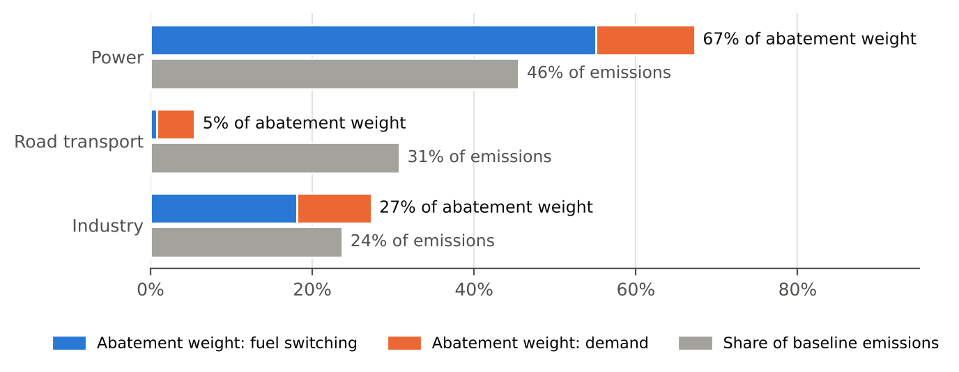
The weights belong to the economy, not the policy. They depend on the energy balance, delivered prices, emission factors and two elasticities per sector, and they are computed once per country and year. Any package is then evaluated by one weighted sum, transparently and reproducibly, and its TECP splits additively by sector, by margin and by instrument. In the worked example (Figure 1), power holds 46 percent of emissions but 67 percent of the abatement weight, industry 24 and 27 percent, and road transport 31 percent of emissions but 5.5 percent of the weight, because a dollar per tonne barely moves the price of motor fuel and fuels in transport emit similar amounts per dollar. Fuel switching carries 74 percent of the weight and demand 26 percent.
2.Source/make_wp_figures.py.
Proposition 2 (the switching margin conserves energy service). (i) Under Proposition 1, for any policy, the switching margin leaves each sector’s service aggregate unchanged to first order: \(\sum_f s_{fs}\,\tilde\varepsilon^{\,\mathrm{int}}_{fs}\,\tau^{\mathrm{int}}_{fs} = \sigma_s\sum_f s_{fs}(\pi_{fs} - \bar\pi_s) = 0\), and for a uniform tax \(\sum_f s_{fs}\tilde\varepsilon^{\,\mathrm{int}}_{fs} = 0\). (ii) Where fuels in a sector have equal prices per unit of service, the switching margin under a uniform tax conserves physical energy: \(\sum_f q_{fs}\tilde\varepsilon^{\,\mathrm{int}}_{fs} = 0\).
The proof is in Appendix B. The economics is that switching moves along an isoquant: at baseline prices, what a sector saves on the fuels it uses less of it spends on the fuels it uses more of. Any change in the scale of energy use belongs to the demand margin. Proposition 2 is a test that any implementation should pass: a switching semi-elasticity that applies the own-price elasticity holding total energy fixed, \(-\sigma_s(1 - s_{fs})\), to a price change already measured relative to the sector average drops the cross-price effects and fails it. Earlier versions of this paper made that error; Appendix E shows its size, a first-order TECP for the example’s mix of $31.7 rather than $33.2.
The decomposition by margin explains why instruments with the same shadow price differ. Write \(\Lambda = \Lambda^I + \Lambda^X\) for the switching and demand parts and \(\omega = \Lambda^I/\Lambda\). Every TECP splits into a switching part and a demand part, \(\tau^* = \omega\,\tau^*_I + (1-\omega)\,\tau^*_X\), where the switching-margin price \(\tau^*_I = \sum_{f,s}E_{fs}\tilde\varepsilon^{\,\mathrm{int}}_{fs}\tau^{\mathrm{int}}_{fs}/\Lambda^I\) and the demand-margin price \(\tau^*_X\) are the policy’s average intensive and extensive prices, weighted by abatement. Computed for one sector, \(\tau^*_{I,s}\) is the sector’s price signal for cleaner production, the quantity border recognition needs (Section 10). A revenue-neutral feebate works almost only on the switching margin, a uniform tax per unit of energy works only on the demand margin, and a renewable subsidy has a negative demand-margin price because it lowers the cost of energy.
Corollary 1 (feebates and same-product routes). A feebate at rate \(t\) around benchmark \(\bar e_s = \sum_f w_{fs}e_f\) changes prices by \(\Delta p_{fs} = t(e_f - \bar e_s)\). Its intensive price is \(\tau^{\mathrm{int}}_{fs} = t - t\,\bar e_s\big(1/p_{fs} - \sum_g s_{gs}/p_{gs}\big)/(x_{fs} - \kappa_s)\). It equals \(t\) for every fuel, and the extensive price is zero, if and only if the fuels or routes have equal prices per unit of service, as competing routes making the same product do.
So the statement that a sector’s switching-margin price equals its feebate rate holds where routes make the same product at the same price, such as steel from blast furnaces and electric arc furnaces, and only approximately elsewhere. A feebate across fuels with different prices per unit, such as road fuels, has an intensive price that differs from \(t\) fuel by fuel and a small nonzero demand-margin price.
The TECP can be stated at any horizon. Because the switching margin adjusts slowly and the demand margin fast, short-run and long-run TECPs weight the margins differently.
Corollary 2 (horizon TECP). Under the partial adjustment of equation 5, the first-order TECP at horizon \(T\) is Proposition 1 with \(\sigma_s\) and \(\eta_s\) replaced by \(a^I_s(T)\sigma_s\) and \(a^X_s(T)\eta_s\), both in the policy’s cut and in the benchmark tax’s. With common speeds across sectors, \[ \tau^*_T = \omega_T\,\tau^*_I + (1 - \omega_T)\,\tau^*_X, \qquad \omega_T = \frac{a^I(T)\,\omega}{a^I(T)\,\omega + a^X(T)\,(1-\omega)} . \tag{10}\]
In the example, the switching margin’s long-run share of the weight is 74 percent and, after one year, 36 percent. An instrument that works by switching, such as a feebate, a renewable subsidy or a fuel standard, therefore has a short-run TECP well below its long-run TECP relative to a tax. The long-run TECP says what a maintained package delivers; the short-run TECP says what it delivers before capital turns over. Both compare a policy with a uniform tax that has had the same time to work.
6 Beyond first order
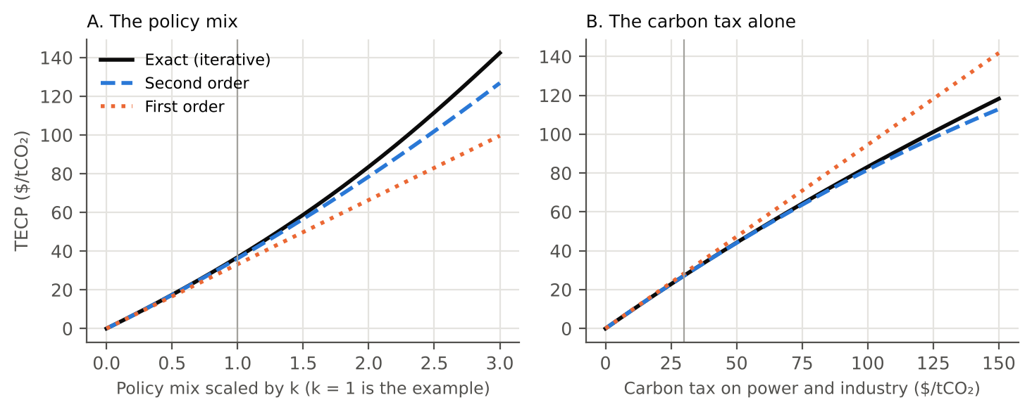
The first-order TECP is a ratio of two linear approximations, so its errors partly cancel. The full CES response is curved: each further dollar of tax cuts less, because the dirtiest fuel’s share shrinks. In the example’s policy mix, the carbon tax raises the delivered price of coal in industry by 71 percent and of coal power by 41 percent. Linearized, the mix cuts 53 Mt; in the full model, 41 Mt. A linear approximation of a cut that large is poor. But the TECP divides the policy’s linear cut by the uniform tax’s linear cut, and both overstate in similar proportion. The first-order TECP of the mix, $33.2, is 10 percent below the exact $36.9; that of the carbon tax alone, $28.4, is 4 percent above the exact $27.2.
Proposition 3 (exact and second-order TECP). (i) The uniform-tax cut \(R(\tau)\) is strictly increasing, with \(R'(\tau) = \sum_s X_s(\tau)\big[\sigma_s V_s(\tau) + \eta_s\kappa_s(\tau)^2\big]\) evaluated at taxed prices and quantities. So the TECP of Definition 1 exists and is unique for any cut in the range of \(R\), which is every cut smaller than baseline emissions when \(\eta_s > 0\) in every sector, and it is found by bisection. (ii) To second order in the price changes, the policy’s cut is \(R_P = R^{(1)}_P + R^{(2)}_P\) with \[ R^{(2)}_P = -\sum_s\sum_f E_{fs}\Big\{\tfrac12\big[\sigma_s\pi_{fs}^2 - (\sigma_s - \eta_s)\big(\bar\pi_s^2 + \sigma_s V^\pi_s\big)\big] + \tfrac12 L_{fs}^2\Big\}, \tag{11}\]
where \(V^\pi_s = \sum_f s_{fs}(\pi_{fs} - \bar\pi_s)^2\) and \(L_{fs} = -\sigma_s\pi_{fs} + (\sigma_s - \eta_s)\bar\pi_s\), and the second-order TECP is \[ \tau^*_{(2)} = \tau^*_{(1)} + \frac{R^{(2)}_P - \tfrac12\,\Gamma\,\big(\tau^*_{(1)}\big)^2}{\Lambda}, \qquad \Gamma = R''(0), \tag{12}\]
with error of third order. (iii) The first-order TECP is exact to second order if and only if the policy’s cut curves as much as that of the uniform tax with the same first-order cut: \(R^{(2)}_P = \tfrac12\Gamma(\tau^*_{(1)})^2\).
Part (iii) says when the linear formula is good enough. For a carbon tax with partial coverage, the policy’s curvature resembles the benchmark’s and the first-order TECP is close. For a mix that adds a subsidy, whose cut grows faster than linearly as the clean fuel’s price falls, the curvatures differ and the first-order TECP understates. Both \(R^{(2)}_P\) and \(\Gamma\) are closed-form sums over the same cells as \(\Lambda\), so the correction costs no more than the first-order formula and should always be reported beside it. In the example \(\Gamma\) is negative, \(-0.042\) Mt per ($/t)², the curvature of diminishing returns.
2.Source/make_wp_figures.py.
The second-order correction removes most of the error over the range that matters. Figure 2 scales the example’s mix and, separately, the carbon tax. For the mix, the first-order error is 5 percent at half the example’s instruments, 10 percent at the example and 20 percent at twice it; the second-order error is 0.4, 1.7 and 6 percent. For the tax alone, the first-order TECP overstates by 4 percent at $30 and 14 percent at $100; the second-order is within 2 percent up to $100. The practical rule follows. Use the first-order formula for weights, decompositions and ranking packages. Report the second-order TECP as the headline when its correction exceeds about 5 percent. Use the exact TECP, by bisection on equation 3, when the correction exceeds about 10 percent or when the number will settle a payment.
Exact TECPs do not add across instruments, and the first-order ones do. In the example the three instruments’ stand-alone exact TECPs sum to $32.7 while the mix’s is $36.9, although the instruments’ exact cuts nearly add (41.0 Mt alone against 40.7 Mt together). The gap comes from the benchmark: each further tonne needs a higher uniform tax, so a cut made of several instruments maps to a higher tax than the sum of their separate equivalents. The convention used here is to report the package’s exact TECP and to attribute it to instruments by their first-order contributions, which add up and are scaled to the exact total.
7 Non-price instruments
A binding rule has no rate but has a shadow price, and the TECP needs either that price or the rule’s emission effect. Standards, mandates, procurement rules and legal obligations cut emissions without a per-tonne charge. They enter the TECP by one of two routes. The shadow-price route converts the rule into the price changes it causes and applies Proposition 1 or Definition 1. The back-out route takes the rule’s emission effect from a model or an evaluation and finds the uniform tax that delivers the same cut. This section sets out when each route applies and what it assumes.
Proposition 4 (tradable standards). Let a sector face a binding intensity standard \(\sum_f e_f q_{fs} \le \bar e^{\,\mathrm{std}}\sum_f q_{fs}\), with credits traded competitively at price \(\lambda\) per tonne and compliance costs passed through to fuel prices. Then (i) the sector’s choices are those of a cost-minimizer facing prices \(p_{fs} + \lambda(e_f - \bar e^{\,\mathrm{std}})\): the standard is a feebate at rate \(\lambda\) with benchmark \(\bar e^{\,\mathrm{std}}\); (ii) its first-order TECP is Proposition 1 with \(\Delta p_{fs} = \lambda(e_f - \bar e^{\,\mathrm{std}})\), and its exact TECP is Definition 1 with \(\lambda\) solving the binding constraint in equation 3; (iii) the shadow-price route and the back-out route give the same exact TECP; (iv) a renewable portfolio standard requiring a clean share \(\theta\), with credits at \(\lambda\) per unit of clean output, is the case \(\Delta p = \lambda\theta\) on each fossil unit and \(-\lambda(1-\theta)\) on each clean unit.
The proof compares first-order conditions (Appendix B). Because the standard binds, average intensity after the policy equals the benchmark, so the implicit feebate is revenue-neutral at the post-policy fuel mix, like the feebates of the series (Stretton 2026c). With competitive trading, each supplier’s marginal cost of compliance equals the credit price (Montgomery 1972), so the credit price is the shadow price of the constraint, and the low-carbon fuel standard’s implicit tax on high-carbon fuel and subsidy to low-carbon fuel (Holland et al. 2009) is exactly a feebate. Part (iv) reproduces Fischer and Newell (2008)’s decomposition of a portfolio standard into a small fossil output tax and a larger renewable subsidy. Because it charges every fossil unit the same, it does not separate coal from gas, and the TECP shows the cost of that in a low switching-margin price.
Identification. The credit price measures the shadow price under four conditions. The market is competitive and clears; if a price ceiling or compliance payment binds, the ceiling is the shadow price. Banking and borrowing allow intertemporal arbitrage, so the price reflects the marginal cost of the path, not only the current year. Pass-through to delivered prices is complete, or its rate is known. The standard’s coverage is known, so the price is applied only to covered fuels. A standard that does not bind has a credit price of zero and a TECP of zero, which is the right answer.
Proposition 5 (non-tradable standards). Let firms \(i = 1, \dots, m\) in a sector each face their own binding standard, with shadow price \(\mu_i\) per tonne, the marginal cost of compliance. Let \(E_i\) be firm \(i\)’s emissions and \(r_i\) its first-order cut per tonne of its emissions per $1 of a feebate at its own benchmark, and write \(\Lambda^F = \sum_i E_i r_i\). Then to first order (i) the standard’s TECP is \[ \tau^* = \frac{\sum_i E_i\, r_i\, \mu_i}{\Lambda} = \frac{\Lambda^F}{\Lambda}\Big[\bar\mu_E + \frac{\mathrm{Cov}_E(r, \mu)}{\bar r}\Big], \tag{13}\]
where \(\bar\mu_E\) is the emission-weighted mean shadow price, \(\bar r\) the emission-weighted mean responsiveness and \(\mathrm{Cov}_E\) the emission-weighted covariance; (ii) if firms are equally responsive per tonne, the TECP is the emission-weighted average marginal compliance cost scaled by \(\Lambda^F/\Lambda\), the sector feebate’s abatement per dollar relative to a uniform tax’s; (iii) a tradable standard that achieves the same cut has the same TECP and a resource cost no higher.
Each firm under its own standard behaves as if it faced a feebate at its own shadow price, so the sector’s cut is the sum of firm-level feebate responses (Appendix B). The covariance term matters. A regulator that reports the simple average compliance cost overstates the TECP if the firms with the highest marginal costs are also the least responsive, which is common: high marginal costs often mean few options. As an illustration, with equal emissions, shadow prices of $100 and $300 per tonne and the high-cost firm half as responsive, the responsiveness-weighted mean is $167, not $200. Part (iii) is a reminder that the TECP measures abatement: a regulator that imposes a cut at needlessly high cost gets no credit for the cost.
Identification. Proposition 5 needs firm-level marginal compliance costs, usually from the regulator’s impact assessment, and firm-level responsiveness, which the CES gives from each firm’s fuel mix and prices. Engineering estimates of compliance costs often report averages; the proposition needs marginal costs. Where only a sector-wide average cost per tonne is available, the back-out route is safer.
Mandates, procurement rules and legal obligations are scored by the emission effect they cause. Many rules change technology choices directly, with no price to observe: a mandate to retire coal plants, a rule that public works use low-carbon cement, building codes, or the forward-announced obligations on energy suppliers in the consumption track of paper 1.1 (Stretton 2026d). For these the TECP is backed out: \(\tau^* = R^{-1}(\Delta E_P)\) exactly, or \(\Delta E_P/\Lambda\) to first order, where \(\Delta E_P\) is the rule’s effect on emissions.
Identification. The backed-out TECP is only as good as \(\Delta E_P\), which must satisfy four assumptions. (A1) Common baseline and horizon: \(\Delta E_P\) is measured against the counterfactual used for \(R(\tau)\), with all other instruments in place, at the same horizon. (A2) Net effect: \(\Delta E_P\) is net of rebound and of leakage within and outside the regulated market. When some US states limited greenhouse gases per mile of new cars inside the federal fuel-economy standard, leakage to the other states offset an estimated 70–80 percent of the reductions from new cars in the adopting states (Goulder et al. 2012). (A3) Consistent behavior: if \(\Delta E_P\) comes from a model, its demand responses must agree with the \(\sigma_s\) and \(\eta_s\) behind \(R(\tau)\); otherwise the TECP compares two models, not two policies. (A4) Causal attribution: an ex post evaluation must identify the rule’s effect against a counterfactual, not before-and-after emissions.
Under a binding cap, an overlapping instrument’s TECP is zero, and the cap’s TECP is the whole effect. If an emissions trading system caps a sector’s emissions and the cap binds, a renewable subsidy or standard inside the capped sector lowers the permit price but not emissions. The rule is then scored at zero, and the cap is scored by backing out the cut from the cap against the baseline, or to first order through the permit price, which is the cap’s shadow price. A package of a cap and complementary rules has the TECP of the cap. This is the waterbed effect, and the metric handles it only if the user applies (A1) with the cap in place.
8 Calibration and uncertainty
Two elasticities per sector drive the weights, and the literature pins them down only to ranges. Table 2 gives the long-run ranges used here, the central values of the worked example and the sources, each cited only for what it estimates. Appendix A, Table A1, gives the evidence by sector and fuel.
| Parameter | Power | Road transport | Industry | Evidence |
|---|---|---|---|---|
| \(\sigma_s\), long run: range (central) | 1.5–3.0 (2.0) | 0.5–1.5 (1.5) | 0.5–1.5 (0.8) | Clean versus dirty energy inputs: significantly above 1 (Papageorgiou et al. 2017). Among fossil fuels, sector estimates below 1 (Serletis et al. 2010). Industry: most fuel pairs above 1, coal pairs imprecise; lower at the macro level (Stern 2012) |
| \(\eta_s\), long run: range (central) | 0.2–0.5 (0.2) | 0.3–0.8 (0.4) | 0.3–0.7 (0.3) | Own-price demand elasticities, long run: CPAT’s reproduction of the 2017 meta-analysis, electricity 0.37–0.51, gasoline 0.53–0.77, diesel 0.39–0.44, industry 0.51 (World Bank and International Monetary Fund 2022; Labandeira et al. 2017); the authors’ own global means, electricity 0.69, gasoline 0.72, diesel 0.60 (Labandeira et al. 2016); gasoline after correcting for publication bias 0.31 (Havranek et al. 2012) |
| \(\lambda^X\), demand adjustment per year | 0.25–0.40 (0.35) | same | same | Ratio of short- to long-run demand elasticities: 0.29–0.34 for energy, electricity, gasoline and diesel in the authors’ own meta-analytic means (Labandeira et al. 2016); about 0.29 for gasoline after bias correction (Havranek et al. 2012) |
| \(\lambda^I\), switching adjustment per year | 0.04–0.10 (0.07) | same | same | Capital turnover: vehicles 6.7 percent a year, buildings 1.2–1.8 percent, in the IMF’s turnover models (Black et al. 2022, Annex C); boilers, furnaces and plants in between |
Each source supports one column, and an older calibration cited them for more. Stern’s meta-analysis covers interfuel substitution in industry, manufacturing and the whole economy, not power, transport or buildings (Stern 2012). Labandeira and coauthors estimate own-price demand elasticities, not substitution elasticities (Labandeira et al. 2017). Sector-level evidence on substitution among fossil fuels finds elasticities below one (Serletis et al. 2010). A power-sector \(\sigma\) of 2 or more is defensible only for substitution between clean and dirty generation, where nested-CES estimates exceed one (Papageorgiou et al. 2017), and that is the nest the example’s power sector represents: coal and gas against renewables. Calibration must also respect the CES structure. A fuel’s total own-price elasticity is \(-\sigma_s + (\sigma_s - \eta_s)s_{fs}\), so an estimate for one fuel identifies \(\sigma_s\) and \(\eta_s\) only jointly with the cost shares; for a dominant fuel it is close to \(-\eta_s\), for a minor fuel close to \(-\sigma_s\).
Errors common to every elasticity largely cancel from the TECP; errors in demand elasticities alone do not. The first-order TECP is a ratio of two cuts, the policy’s and the benchmark tax’s, each linear in the elasticities. Scaling every \(\sigma_s\) and \(\eta_s\) by the same factor scales both and leaves the first-order TECP unchanged. Scaling only the demand elasticities shifts weight from the switching margin to the demand margin, and changes the TECP of any policy whose mix of margins differs from a uniform tax’s. That is the relevant case: meta-analytic demand elasticities are biased upward in magnitude, and correcting for selective reporting roughly halves the mean gasoline price elasticity, from about −0.23 to −0.09 in the short run and from −0.69 to −0.31 in the long run (Havranek et al. 2012). The example’s mix leans on switching (the subsidy and the fuel standard act through relative prices), so overstated demand elasticities make the benchmark tax look more effective and lower the mix’s TECP. Table 3 shows the size: halving every demand elasticity raises the exact TECP from $36.9 to $40.2; doubling them lowers it to $32.7; halving every elasticity, substitution included, leaves it at $37.1.
2.Source/tecp_model.py.
| Calibration | Demand elasticities: power, road, industry | TECP, first order ($/t) | TECP, exact ($/t) |
|---|---|---|---|
| Central case | 0.20, 0.40, 0.30 | 33.2 | 36.9 |
| Every elasticity at the midpoint of its range | 0.35, 0.55, 0.50 | 32.4 | 35.2 |
| CPAT’s demand elasticities (paper 5.4) | 0.53, 0.58, 0.66 | 31.5 | 33.1 |
| CPAT’s demand elasticities halved (paper 5.4) | 0.27, 0.29, 0.33 | 33.3 | 37.0 |
| Demand elasticities halved | 0.10, 0.20, 0.15 | 34.6 | 40.2 |
| Demand elasticities doubled | 0.40, 0.80, 0.60 | 31.2 | 32.7 |
| Every elasticity halved | 0.10, 0.20, 0.15 | 34.2 | 37.1 |
| Monte Carlo, 5th–95th percentile (median) | Drawn from Table 2 | 31.3–33.4 (32.4) | 32.4–38.1 (35.3) |
The central case sits toward the top of the band, and paper 5.4’s alternatives sit inside it. Because the example’s demand elasticities for power and industry are at the bottom of their ranges, its exact TECP, $36.9, exceeds the Monte Carlo median of $35.3; with every elasticity at the midpoint of its range it is $35.2. Paper 5.4, which checks CPAT’s elasticities against the evidence, ran this paper’s model with CPAT’s demand elasticities, at or just above the top of the ranges in Table 2, and found $33.1, near the bottom of the band; halving them, the publication-bias correction for gasoline, gives $37.0 (Stretton 2026a). The two papers therefore agree: elasticity errors of the size the evidence allows move the example’s TECP by about a tenth, much less than they move estimated emission cuts, which rise by about a third under CPAT’s demand elasticities. The central case is kept because the series quotes it.
2.Source/make_wp_figures.py.
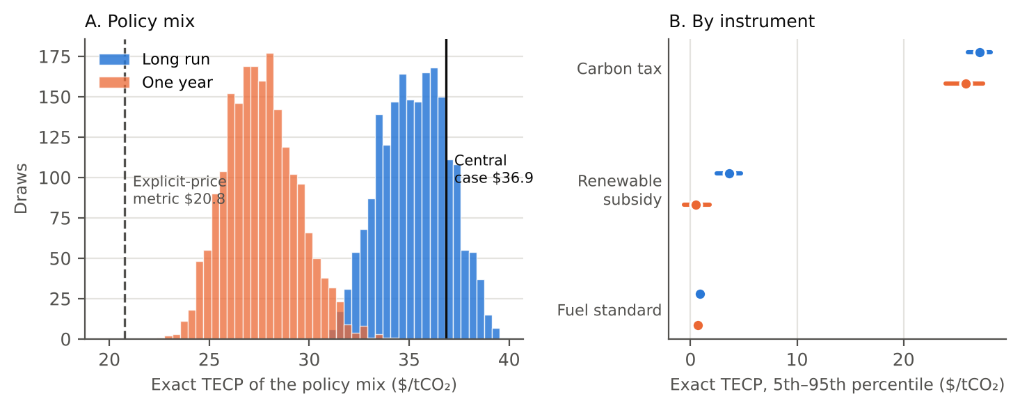
Carried through the model, the elasticity uncertainty gives a band of $32–38 per tonne for the example’s mix in the long run. Figure 3 shows 2,000 draws. The long-run exact TECP of the mix has a median of $35.3 and a 90 percent range of $32.4–38.1; the first-order TECP, $31.3–33.4. After one year the exact TECP is $24.8–30.7. In every draw, long run or one year, the TECP exceeds the explicit-price metric’s $20.8. The band is narrow relative to the elasticity ranges because the TECP is a ratio, so what moves it is the relative responsiveness of sectors and margins. The fuel standard’s credit price is far more uncertain, $171–382 per tonne, because a fixed intensity target costs more to meet when substitution is harder; its TECP stays at $0.7–1.1. The band covers elasticity uncertainty only, not model structure, data errors or the salience question below.
Taxes may move demand more than equal market price changes, and a price-elasticity calibration then understates explicit taxes. Several studies find that fuel demand responds more to tax changes than to equal changes in tax-exclusive prices: in US states, consumers respond more strongly to gasoline tax changes than to other price changes (Li et al. 2014); in Sweden the carbon-tax elasticity of gasoline demand was three times the price elasticity (Andersson 2019); and instrumental-variable estimates that exploit US tax changes imply that a 10-cent-per-gallon tax rise cuts vehicle CO₂ by about 1.5 percent, more than least-squares price elasticities suggest (Davis and Kilian 2011). If taxes are more salient, the uniform tax that defines the TECP is more effective than a price-calibrated \(\Lambda\) says, and non-tax instruments, whose price wedges reach buyers as ordinary price changes, are worth less in units of it. Applying a salience factor of 3, the Swedish estimate, to the demand margin of taxes only, the example’s subsidy falls from $3.7 to $2.4 and the fuel standard from $1.2 to $0.8 at first order, and the mix from $33.2 to $30.3. The evidence comes from road fuels, and its persistence and transfer to other sectors are open. A user who adopts it should state the factor and apply it only to the price changes that come from taxes.
9 A worked example
A stylized economy shows how far the TECP and the existing metrics diverge. The economy has three sectors with 261 Mt of baseline CO₂ (Appendix D, Table 5): power, with coal, gas and renewables (119 Mt); road transport, with gasoline, diesel and biofuel (80 Mt); and industry, with coal, oil and gas (62 Mt). Delivered prices include existing taxes. Elasticities are the central values of Table 2. All numbers are stylized; the brief uses the same economy and reports the same results.
The policy mix has a tax, a subsidy and a standard. A carbon tax of $30 per tonne covers power and industry. A subsidy of $10 per MWh goes to renewable generation. A tradable low-carbon fuel standard requires road fuels’ carbon intensity per unit of energy to fall 2 percent below its baseline; in the full model it binds at a credit price of $166 per tonne. A uniform tax of $1 per tonne on every fuel cuts emissions by 1.59 Mt, 0.61 percent.
2.Source/make_wp_figures.py.
| Instrument | Rate or shadow price | Explicit-price metric | Comprehensive carbon price | TECP, first order: switching + demand | TECP, first order | TECP, exact | Exact, 90% range | Exact, after one year |
|---|---|---|---|---|---|---|---|---|
| Carbon tax, power and industry | $30/t | 20.8 | 20.8 | 22.0 + 6.4 | 28.4 | 27.2 | 26.0–28.2 | 25.4 |
| Renewable subsidy | $10/MWh | 0 | 0 | 4.1 − 0.4 | 3.7 | 4.3 | 2.5–4.7 | 1.2 |
| Low-carbon fuel standard, −2% | $166/t credit price | 0 | 51.1 | 1.0 + 0.2 | 1.2 | 1.2 | 0.7–1.1 | 0.8 |
| Policy mix | 20.8 | 71.8 | 27.1 + 6.1 | 33.2 | 36.9 | 32.4–38.1 | 28.3 |
The TECP rates the mix at $33 per tonne to first order and $37 exactly; the explicit-price metric says $21. Table 4 sets out the comparison. The tax alone is worth $27–28, not $21, because the explicit-price metric divides it over transport’s 31 percent of emissions, which hold only 5.5 percent of the abatement weight. The renewable subsidy adds $3.7 to first order: $4.1 through switching, less $0.4 because cheaper power raises demand. The fuel standard binds at $166 per tonne and adds $1.2. Counting its credit price as a carbon price on the emissions it covers, as the comprehensive carbon price does, puts the mix at $72: a high price on a large, unresponsive base. The subsidy’s budgetary cost per tonne avoided is $79 ($514 million on 51 TWh of renewable output for a cut of 6.6 Mt), so an average-cost implicit price would rank it as the most ambitious instrument in the mix; its TECP ranks it a distant second.
The IMF’s equivalence approach and the exact TECP coincide when they use the same model. Re-simulating the mix and searching for the matching uniform price, as Black et al. (2022) do in CPAT, gives $36.9 here because the search runs on the same CES. The first-order TECP reaches $33.2 with one weighted sum and the second-order $36.2 with two. What the closed form adds is the decomposition: 82 percent of the mix’s first-order TECP comes through fuel switching, and almost all of that in power and industry.
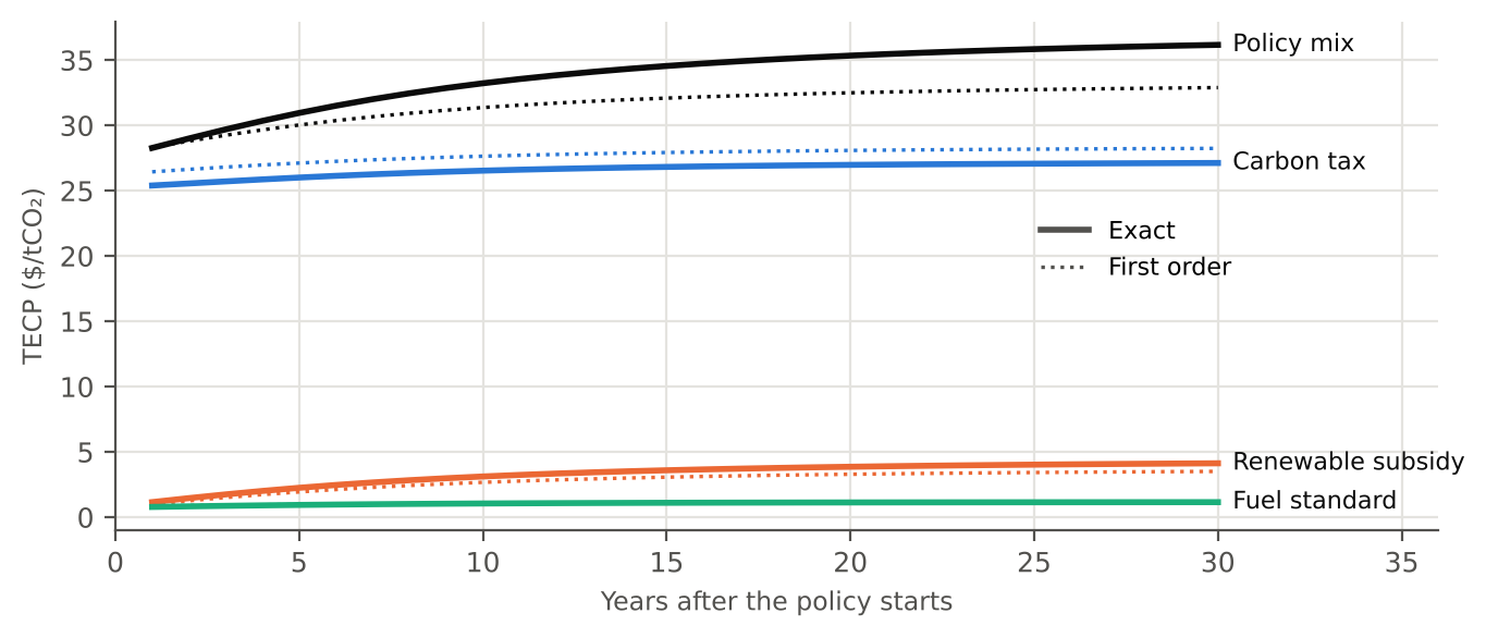
The mix is worth $28 after one year and $37 in the long run. Figure 4 shows the TECP by horizon under the central adjustment speeds. After one year the subsidy is worth $1.2, a quarter of its long-run value, because new renewable capacity takes time while the demand response to cheaper power comes quickly. The carbon tax is worth $25.4 after a year against $27.2 in the long run, less of a gap because the demand response it triggers is fast. The mix reaches $33 after ten years. A country that announces this package can claim a long-run TECP of $37, but in the first years it delivers what a $28–31 uniform tax would. A model that applies the full long-run response in the year a price changes, as CPAT does (World Bank and International Monetary Fund 2022; Stretton 2026a), would report $37 for the first year too, about 30 percent above the one-year value.
2.Source/make_wp_figures.py.
10 Uses
Policy crediting needs a common unit, and the TECP supplies it. Paper 1.1 shows that if an outside buyer pays \(\pi\) per tonne abated, a feebate at rate \(t\) is a net gain for the adopting country whenever \(\pi > t/2\), and the country’s best response is \(t = \pi\) (Stretton 2026d, Prop. 6). Paying for policies rather than projects requires measuring the tonnes a policy cuts, separately from changes in output and fuel prices. The TECP does this: the tonnes credited for a policy change are \(R(\tau^*_{\text{after}}) - R(\tau^*_{\text{before}})\) in the full model, or \(\Lambda\,\Delta\tau^*\) to first order. A country that adopts a fuel standard or a procurement rule then earns the same payment per tonne as one that adopts a tax. Because the TECP is a forecast, payments should be settled against observed emissions, and the “change from a benchmark year” design of the IMF price-floor proposal (Parry, Black, and Roaf 2021) avoids paying for instruments set long ago for other reasons.
For border recognition, the sector’s switching-margin price measures the signal to credit. The EU’s border mechanism reduces an importer’s charge by the carbon price “effectively paid” in the country of origin, net of rebates and compensation (European Parliament and Council of the European Union 2023; European Parliament and Council of the European Union 2025, Art. 9). A feebate, a rebated tax or an intensity standard pays almost nothing net, so it earns nothing, although its marginal signal is the full rate (Stretton 2026b, Prop. 4). Paper 1.4 proposes a liability that credits the country-sector price signal alongside the price paid (Stretton 2026b). The TECP’s switching-margin price for the sector, \(\tau^*_{I,s}\), is that signal for price and non-price instruments alike: a feebate across routes that make the same product scores its rate (Corollary 1), a tradable standard its credit price (Proposition 4), and a fuel tax or subsidy its per-tonne rate weighted by how strongly the sector’s fuel use responds. The demand margin is left out because the border charge is on embodied carbon and the demand response in the importing market comes from the importer’s own price. Two cautions apply. Equal emission effects are not equal costs: a regulation at a given shadow price imposes lower private costs on firms than a tax at the same rate, because there is no tax payment on remaining emissions (Keen et al. 2022; Black et al. 2022, Annex B). So recognition on the TECP rewards effort, not competitive burden, and the importer’s producers can fairly ask which is being matched. And border credit traditionally rests on average prices paid, while the TECP is a marginal measure (Agnolucci et al. 2024).
For country diagnostics, the decomposition is the product. The TECP shows which sectors and margins a package reaches and which it misses. In the example, extending the $30 tax to road fuels would add only about $1.6 to the TECP, because transport holds 5.5 percent of the abatement weight. The package’s weak point is the low responsiveness of road transport to any carbon price at the margin, which argues for instruments aimed at vehicle choice rather than a higher fuel price. Computed each year from the energy balance, the TECP gives one trajectory for a country’s effective carbon price against which announced packages, nationally determined contributions and price-floor commitments can be checked. Published weights also let others reproduce the number, which J. E. Aldy and Pizer (2016) identify as a requirement for any metric of comparable effort.
Computing the TECP for a country needs four inputs that statistical offices and international agencies already hold. The first is an energy balance by fuel and sector, such as the International Energy Agency’s world energy balances. The second is delivered prices including taxes and subsidies, from national statistics or the fuel-price data behind the World Bank’s total carbon price and the IMF’s subsidy estimates (Agnolucci et al. 2024; Black, Liu, et al. 2023). The third is emission factors per unit of fuel. The fourth is the two elasticities per sector, from the ranges in Table 2 or a country study. From these, \(X_s\), \(\kappa_s\) and \(V_s\) follow by sector, and \(\Lambda\) and the weights by equation 8 and equation 9. Each instrument is then entered as the price changes it causes; standards through their credit or shadow prices; mandates through their evaluated effect. The scripts in 2.Source/ do this for the stylized economy and take a country’s data in the same format.
11 Limits
The paper has no real-country application yet. The worked example shows the mechanics and the size of the gap between explicit and effective prices in a plausible economy, not in any actual one. The gap depends on how much of a country’s explicit pricing falls on responsive sectors and how much of its policy works through standards and subsidies; both vary widely. Until the TECP is computed for real countries and compared with the IMF’s model-based equivalents, the $21 against $37 contrast is an illustration.
The TECP measures abatement, not cost or welfare. Two packages with the same TECP cut the same tonnes; they need not cost the same. Per tonne, standards and subsidies generally cost more than a price (Fischer and Newell 2008), static costs per tonne vary widely across instruments (Gillingham and Stock 2018), and subsidies without carbon pricing can raise mitigation costs several-fold (Kalkuhl et al. 2013). Replacing a feebate with a tax of equal TECP is not welfare-neutral either: interactions with the existing tax system differ, and a clean energy standard can cost less than emissions pricing for small cuts because it is a smaller implicit tax on factors of production (Goulder et al. 2016). The TECP should be reported beside each instrument’s shadow price and cost, never instead of them.
Overlapping instruments do not simply add. First-order TECPs add by construction, but emission effects interact. Within a binding cap, complementary instruments add nothing (Section 7). Nested regulations leak, sometimes most of their effect (Goulder et al. 2012). The TECP of a package should come from the package’s joint effect, with instrument attribution as a second step.
The model is partial and static in technology. It holds incomes, other sectors and the supply of fuels fixed. It does not capture links between sectors, such as the power demand created by electric vehicles, except through the prices the user enters. It credits a solar subsidy only for current abatement, not for the cost declines it may induce (Gillingham and Stock 2018), and it ignores fossil-fuel supply responses, through which a badly designed subsidy can raise emissions over time (Kalkuhl et al. 2013).
The inputs inherit the problems of measuring prices. The intensive and extensive prices come from instrument rates and fuel prices that are hard to measure in many countries. Price-gap estimates confuse market power and distribution costs with taxes, and fuel taxes set for revenue or congestion should not be relabeled as carbon prices (Agnolucci et al. 2024; Parry, Black, and Roaf 2021). The TECP improves the weighting, not the measurement of what is weighted.
Shadow prices can be gamed. A government that reports its standards’ shadow prices has reason to overstate them. Tradable standards have observable credit prices; for non-tradable rules, the back-out route with an independent evaluation is the safer basis, and an independent body could compute TECPs for all countries from a common elasticity set.
12 Conclusion
A policy mix is worth the uniform carbon tax that would cut emissions as much, and that number can be computed from an energy balance and two elasticities per sector. The CES derivation gives switching and demand semi-elasticities whose weights have a simple form: spending times the substitution elasticity times the dispersion of carbon per dollar, plus the demand elasticity times carbon per dollar squared, and the switching margin conserves energy service. A second-order correction makes the closed form accurate to within a few percent for packages that raise some fuel prices by more than half, and the exact value follows by bisection. Tradable standards enter at their credit price, non-tradable ones at a responsiveness-weighted average of marginal compliance costs, and mandates through their modeled effect, each under stated assumptions. In a stylized economy the metric rates a mix at $37 per tonne in the long run, $32–38 across calibrations and $28 after one year, where explicit-price metrics say $21 and the comprehensive carbon price $72. Errors common to all elasticities cancel, but demand elasticities alone move the number: with CPAT’s it is $33. The main limitations are the absence of a real-country application and calibration: substitution elasticities outside industry rest on thin evidence, and taxes may be more salient than prices. The next step is to compute the TECP for a G20 country from its energy balance and to compare it with the IMF’s model-based equivalent for the same policies.
Downloads
References
Appendix A: Literature review
This appendix condenses a fuller review prepared for version 0.3 (5.Notes/LiteratureAppendix-draft.md), re-checked for version 0.4. Each bibliography entry’s note records what was read.
A.1 Price-signal metrics
The effective carbon rate and the total carbon price aggregate prices on a fuel-by-sector grid and weight them by emissions. The OECD’s effective carbon rate is the sum of fuel excise taxes, explicit carbon taxes and emissions trading prices, computed for each fuel and sector and aggregated by emissions; the net rate deducts fossil-fuel subsidies (OECD 2023). It deliberately excludes non-price instruments and does not weight by responsiveness, a point Parry, Black, and Roaf (2021, n. 26) make explicitly. The World Bank’s total carbon price for 142 countries over 1991–2021 sums direct pricing, carbon taxes and trading weighted by coverage, and indirect pricing, fuel excises, consumption subsidies and deviations from standard VAT, measured by a price-gap method (Agnolucci et al. 2024, 2023). Indirect pricing is 87 percent of the global total in 2021, the global average is barely above its 1994 level, transport is priced highest and coal and gas are barely priced. Compared with the OECD’s net rate, the total carbon price is broadly aligned for OECD countries but often far off, sometimes of opposite sign, for poorer countries. Its section 6.4 proposes “effectiveness-weighted total carbon pricing”, weighting by fuel- and sector-specific mitigation elasticities, and section 6.3 notes that border credit rests on average rather than marginal prices. The World Carbon Pricing Database documents explicit instruments by IPCC sector for national and subnational jurisdictions from 1990 (Dolphin and Xiahou 2022), which maps onto the TECP’s sector dimension.
One econometric study estimates how emissions respond to an aggregate effective carbon price. D’Arcangelo et al. (2022) estimate in a large cross-country panel that a €10 rise in the effective carbon rate cuts fossil CO₂ by 3.7 percent in the long run, that broadening coverage to unpriced emissions delivers two thirds of the potential effect, and that responses vary with sectoral structure. This is an external check on \(\Lambda\): the example’s 0.61 percent per dollar per tonne is of the same order as their 0.37 percent per euro.
The IMF’s price-gap estimates measure distance from efficient prices. Efficient fuel prices include supply costs, environmental costs and forgone consumption taxes. Global fossil-fuel subsidies so measured were $5.9 trillion in 2020, 8 percent explicit and 92 percent implicit (Parry, Black, and Vernon 2021), and $7 trillion in 2022 (Black, Liu, et al. 2023); earlier estimates are in Coady et al. (2019). The fuel-demand responses behind these estimates use constant-elasticity curves. An implicit subsidy is a gap to an efficient price, not a policy price, and only the explicit part belongs in the TECP’s cells, as in the World Bank measure. Critics of price-gap methods note that they confuse market power and distribution costs with taxes and that reference prices are hard to set in large countries (Agnolucci et al. 2024, sec. 6.2); the TECP inherits these problems in its inputs.
A.2 Implicit carbon prices of non-price policies
The older meaning of “effective carbon price” is cost per tonne abated. The OECD’s 2013 study estimates the cost per tonne of policies in 15 countries and five sectors, across taxes, trading, feed-in tariffs, capital subsidies and regulations, and finds market instruments consistently cheapest and capital subsidies and feed-in tariffs among the most expensive (OECD 2013, abstract). Marcantonini and Ellerman (2015) compute the net cost of German feed-in tariffs for wind and solar in 2006–2010, divide by CO₂ abated, and add the allowance price: tens of euros per tonne for wind and hundreds for solar. Gillingham and Stock (2018) survey static costs per tonne of standards, mandates and subsidies, which run from negative to several hundred dollars, and argue that static cost can mislead where learning and spillovers lower future costs (abstract). Against these, the TECP is a marginal emissions-equivalence measure: the TECP of German solar support is the uniform tax that would cut as much CO₂, far below its average cost.
Instrument-level studies decompose standards into implicit taxes and subsidies. Fischer and Newell (2008) rank US power-sector instruments by cost for a given cut: an emissions price, a performance standard, a fossil-output tax, a renewable portfolio standard, a renewable production subsidy and research subsidies. Each decomposes into implicit taxes and subsidies by technology; a portfolio standard is a small fossil-output tax with a larger renewable subsidy, no conservation incentive and a slightly lower electricity price. Holland et al. (2009) show that a low-carbon fuel standard taxes high-carbon fuel and subsidizes low-carbon fuel, can in principle raise emissions, and in simulation is costly: an average carbon cost of $307–2,272 per tonne for a national standard cutting carbon intensity 10 percent, against $60–868 for an efficient policy with the same cut. Goulder et al. (2016) show that a clean energy standard, an implicit tax on dirty and subsidy to clean generation, distorts factor markets less than emissions pricing because it is a smaller implicit tax on factors of production, and that this can make it cheaper for small cuts. These results are the TECP’s margin decomposition in other words: instruments with small or negative extensive prices deliver less abatement per dollar of shadow price.
Overlapping and supply-side effects limit any static equivalence. Goulder et al. (2012) find that state limits on greenhouse gases per mile nested inside federal fuel-economy standards cause leakage to other states that offsets 70–80 percent of the reductions from new cars in adopting states. Kalkuhl et al. (2013) show in a general-equilibrium model with fossil-resource owners that renewable subsidies without carbon pricing raise mitigation costs by a multiple, and that small deviations from the second-best subsidy raise emissions sharply through extraction paths.
A.3 Carbon price equivalents and comparing effort
The carbon price equivalent was defined in law and economics before the IMF computed it. Weil (2021) proposes the “carbon price equivalent” as a metric for comparing mitigation effort across jurisdictions: the carbon price that, applied in an otherwise neutral policy environment, would produce the same aggregate emissions as the jurisdiction’s actual mix, or equivalently the allowance price of a cap-and-trade system whose cap matched observed emissions. He argues for it on grounds of justice and efficiency, proposes it for border adjustments of domestic carbon taxes and regulations, and discusses the neutral baseline, currency conversion, production against consumption emissions and spillovers. He does not compute it or give a method that separates margins.
The IMF defines the carbon price equivalent and computes it for the G20. Black et al. (2022) define the carbon price equivalent of a policy as the carbon price that yields the same emissions reduction, with economy-wide and sectoral versions. Their method builds a business-as-usual path in CPAT, simulates the policy or target, and finds the matching price. For the G20 in 2030, explicit pricing gives modest equivalents except about $50 per tonne or more in Canada, France, Germany, Italy and the United Kingdom; power-sector renewable and coal phase-out targets imply sectoral equivalents above $150 in ten cases; all policies combined exceed $150 in six cases; existing fuel taxes imply about $5–40 in most cases, with the question whether they should count left open. Vehicle and building responses come from capital-turnover models with 15-, 55- and 85-year lives. Renewable targets are modeled as a subsidy plus an electricity tax, intensity standards as an output-rebated carbon charge and vehicle standards as a shadow price on efficiency. Their Annex B stresses that equal emissions do not mean equal costs or competitiveness effects. CPAT itself models non-price policies through a shadow price on the efficiency margin only and splits elasticities into usage and efficiency margins calibrated to Labandeira et al. (2017; Black, Parry, et al. 2023; World Bank and International Monetary Fund 2022).
The IMF’s price-floor proposal asks for effectiveness weighting. Parry, Black, and Roaf (2021) propose a floor among six large emitters at $50 per tonne, or $25, $50 and $75 differentiated by income, which would cut energy CO₂ 23–24 percent below the 2030 baseline. It admits “non-pricing approaches with equivalent emissions impacts”. Its compliance metric expresses fuel taxes in CO₂ terms and weights fuel taxes and explicit prices by their relative effectiveness at reducing economy-wide CO₂ compared with a comprehensive carbon price, and it would bind on the increase from a benchmark year, because fuel taxes are set for other reasons. The October 2019 Fiscal Monitor describes the same weighting, CO₂-equivalent fuel taxes and direct carbon prices weighted by their relative effectiveness, and refers to first-pass estimates of effective carbon prices for 135 countries published separately (International Monetary Fund 2019, Box 1.2).
Comparisons of national effort need replicable metrics. J. E. Aldy and Pizer (2016) survey metrics, from emissions and intensity to explicit and implicit prices and costs, and conclude that none is comprehensive, measurable and universal, so a dashboard is needed. Implicit prices estimate average abatement cost, are model-derived and are high both for costly policies and for those that abate little. They call for an economy-wide average carbon price that weights explicit and implicit prices. J. E. Aldy et al. (2017) propose ex ante and ex post review of pledges and show that rankings change with the metric; with four integrated assessment models, J. Aldy et al. (2016) find marginal abatement costs of Paris pledges differing by two orders of magnitude across countries. Model dispersion of this size is why a TECP needs a band.
A.4 Energy demand elasticities, interfuel substitution and adjustment
Own-price demand elasticities are well studied; substitution elasticities outside industry are not. Labandeira et al. (2017) meta-analyze own-price elasticities of energy demand by fuel and sector. As reproduced in the CPAT technical notes, long-run means are about −0.62 residential, −0.51 industrial, −0.72 commercial and −0.44 transport; by fuel, −0.51 for electricity, −0.57 for natural gas, −0.53 for gasoline and −0.39 for diesel, with “adjusted” values of −0.37, −0.68, −0.77 and −0.44 (World Bank and International Monetary Fund 2022). These are CPAT’s reproduction of the meta-analysis, partly adjusted; the authors’ own summary of their global meta-analysis gives larger long-run means, −0.65 for energy, −0.69 for electricity, −0.85 for natural gas, −0.72 for gasoline and −0.60 for diesel, with short-run means about 0.3 times as large (Labandeira et al. 2016). All are demand elasticities. Stern (2012) meta-analyzes interfuel substitution elasticities among coal, oil, gas and electricity in 47 studies of industry, manufacturing and the whole economy, with no power-generation, transport or residential samples. At the level of the industrial sector, the oil–coal, oil–gas, oil–electricity and gas–electricity elasticities are significantly greater than one, the coal–gas and coal–electricity elasticities are imprecise, and substitution is more constrained at the macro level. For a single CES nest every such elasticity equals \(\sigma\), so differences across pairs are evidence against one \(\sigma\) per sector. Serletis et al. (2010) estimate sectoral interfuel elasticities for OECD and developing countries in models with fossil fuels only and find them consistently below one. Papageorgiou et al. (2017) estimate a nested CES on sectoral data for 26 countries and find the elasticity between clean and dirty energy inputs significantly above one (abstract), the relevant nest for power generation with renewables.
Published elasticities are biased upward in magnitude. Havranek et al. (2012) find that published gasoline price elasticities average about −0.23 in the short run and −0.69 in the long run, but that correcting for selective reporting gives −0.09 and −0.31. Meta-analytic means should therefore be treated as upper bounds on responsiveness, and a calibration needs a bias-corrected case.
Taxes move demand more than equal price changes. Davis and Kilian (2011) find small OLS price elasticities for US gasoline, about −0.1 nationally, but larger instrumental-variable estimates exploiting tax changes; their preferred estimate is that a 10-cent tax rise cuts vehicle CO₂ by about 1.5 percent. Li et al. (2014) find that US consumers respond more strongly to gasoline tax changes than to equal changes in tax-exclusive prices. Andersson (2019) finds that Sweden’s carbon tax cut transport CO₂ by almost 11 percent and that its elasticity was three times the price elasticity (abstract). A TECP calibrated to price elasticities therefore understates taxes relative to instruments whose price wedges reach buyers as ordinary price changes (Section 8).
Partial adjustment links short- and long-run elasticities. The Nerlove identity, adjustment speed equals the ratio of short- to long-run elasticity, gives 0.29–0.34 a year from the authors’ own meta-analytic means for energy, electricity, gasoline and diesel (Labandeira et al. 2016) and 0.29 for gasoline from bias-corrected estimates (Havranek et al. 2012). That is the demand margin. For fuel switching, capital turnover sets the pace: CPAT uses vehicle turnover of 6.7 percent a year and slower rates for buildings (Black et al. 2022, Annex C). For non-OECD calibration, country-specific road-fuel elasticities (Dahl 2012) and a review for industrializing economies (Huntington et al. 2019) are the next sources to use; paper 5.4 assembles them into a register by fuel and sector (Stretton 2026a).
| Sector | Demand elasticity, long run | Substitution elasticity | Sources |
|---|---|---|---|
| Road transport | −0.3 (bias-corrected) to −0.8; diesel −0.4 to −0.6 | Weak evidence; 0.5–1.5 at a 10–15-year horizon; fossil fuels only below 1 | Havranek et al. (2012); World Bank and International Monetary Fund (2022); Labandeira et al. (2016); Serletis et al. (2010) |
| Power | Electricity demand −0.37 (CPAT, adjusted) to −0.69 (authors’ mean) | Clean versus dirty above 1; among fossil fuels below 1 | World Bank and International Monetary Fund (2022); Labandeira et al. (2016); Papageorgiou et al. (2017); Serletis et al. (2010) |
| Industry | About −0.5 (coal) to −0.7 (gas) | Most fuel pairs above 1; coal pairs imprecise; macro level lower | World Bank and International Monetary Fund (2022); Stern (2012) |
| Buildings | Gas about −0.65 to −0.76; electricity about −0.36 to −0.42 | Mostly below 1 among fuels | World Bank and International Monetary Fund (2022); Serletis et al. (2010) |
| Economy-wide | About −0.5 to −0.8 | — | Black et al. (2022); Labandeira et al. (2016) |
A.5 Uses: border adjustment, price floors and crediting
The economics of border adjustment separates environmental equivalence from cost equivalence. Keen et al. (2022) show that non-price policies impose only the efficiency cost of abatement on firms, not the payment on remaining emissions, so they “generally impose markedly lower private costs on firms than carbon pricing (at equivalent shadow prices)”. Charging imports the shadow price is then not a competitiveness response, and exemptions for non-price effort are justified on cooperation or leakage grounds rather than competitiveness. Mehling et al. (2019) anticipate adjusting border charges for effective carbon prices, explicit and implicit, computed from energy taxes by carbon content, average abatement cost times mandated reductions, or “economic models to identify the carbon price needed to achieve mandated emission reductions in a sector”, with third-party verification. Cosbey et al. (2019) review design choices. The EU’s mechanism deducts only the carbon price effectively paid, net of rebates and compensation (European Parliament and Council of the European Union 2023; European Parliament and Council of the European Union 2025, Art. 9), and so does not recognize feebates or standards; paper 1.4 proposes recognizing the price signal (Stretton 2026b).
No source found in this review measures policy-level crediting by a carbon-price equivalent. Results-based climate finance pays for verified reductions, mostly by project. The crediting argument of paper 1.1 (Stretton 2026d) pairs the two.
A.6 What is new here
The concept of a carbon price equivalent, the idea of weighting by responsiveness, the counting of standards at their marginal incentive and the representation of standards by shadow prices all precede this paper (Weil 2021; Black et al. 2022; Parry, Black, and Roaf 2021; Carhart et al. 2022; Fischer and Newell 2008; Black, Parry, et al. 2023). What this paper adds is: a closed-form, linear-in-policy TECP whose weights belong to the economy and can be published, with a corrected derivation from the CES cost function; a decomposition of every instrument into a switching and a demand margin; an exact and second-order version with a rule for when the closed form suffices; a theory of non-price instruments with identification assumptions; and a calibration that cites each source only for what it estimates, with an uncertainty band. The main objections a referee will raise are also in the literature: calibration fragility, especially of demand elasticities (Serletis et al. 2010; Havranek et al. 2012), tax salience (Li et al. 2014; Andersson 2019), the difference between emission and cost equivalence (Keen et al. 2022; Goulder et al. 2016), and the failure of additivity under leakage and binding caps (Goulder et al. 2012). Section 8 and Section 11 address each.
Appendix B: Derivations and proofs
All results below were checked symbolically with sympy and numerically against the full nonlinear CES; 2.Source/verify_derivations.py runs the 30 checks.
B.1 Proposition 1
From equation 3, \(\ln q'_{fs} = \ln q_{fs} - \sigma_s\ln P_{fs} + (\sigma_s - \eta_s)\ln(C'_s/C_s)\). At the baseline, \(\partial\ln P_{fs}/\partial\pi_{gs} = \delta_{fg}\) and, by Shephard’s lemma, \(\partial\ln C_s/\partial\pi_{gs} = s_{gs}\). So \(d\ln q_{fs} = -\sigma_s\pi_{fs} + (\sigma_s - \eta_s)\bar\pi_s = -\sigma_s(\pi_{fs} - \bar\pi_s) - \eta_s\bar\pi_s\), which is equation 4. The cut is \(R_P = -\sum_{f,s}E_{fs}\,d\ln q_{fs} = \sum_s\big[\sigma_s\sum_f E_{fs}(\pi_{fs} - \bar\pi_s) + \eta_s E_s\bar\pi_s\big]\). By equation 6, \(\sigma_s(\pi_{fs} - \bar\pi_s) = \sigma_s(x_{fs} - \kappa_s)\,\tau^{\mathrm{int}}_{fs} = \tilde\varepsilon^{\,\mathrm{int}}_{fs}\tau^{\mathrm{int}}_{fs}\) and \(\eta_s\bar\pi_s = \eta_s\kappa_s\,\tau^{\mathrm{ext}}_s = \tilde\varepsilon^{\,\mathrm{ext}}_s\tau^{\mathrm{ext}}_s\), which proves (i). For (ii), a $1 tax gives \(\pi_{fs} = x_{fs}\) and \(\bar\pi_s = \kappa_s\), so \(\tau^{\mathrm{int}}_{fs} = \tau^{\mathrm{ext}}_s = 1\). Since \(E_{fs} = X_s s_{fs}x_{fs}\), \(\sum_f E_{fs}(x_{fs} - \kappa_s) = X_s\big(\sum_f s_{fs}x_{fs}^2 - \kappa_s^2\big) = X_sV_s\), and \(E_s\kappa_s = X_s\kappa_s^2\). So \(\Lambda = \sum_s X_s(\sigma_sV_s + \eta_s\kappa_s^2)\), positive whenever some sector has \(\eta_s > 0\) and positive emissions, or \(\sigma_s > 0\) and \(V_s > 0\). (iii) follows by dividing by \(\Lambda\); the weights sum to \(\Lambda/\Lambda = 1\). (iv) A tax \(\tau\) gives \(\pi_{fs} = \tau x_{fs}\), so both prices equal \(\tau\) and \(R_P = \tau\Lambda\).
B.2 Proposition 2
- \(\sum_f s_{fs}\sigma_s(\pi_{fs} - \bar\pi_s) = \sigma_s(\bar\pi_s - \bar\pi_s) = 0\). At a cost minimum the elasticity of the CES aggregate with respect to each input equals its cost share, so \(d\ln Q_s = \sum_f s_{fs}\,d\ln q_{fs}\) and the switching term contributes nothing to \(Q_s\). For a uniform tax, \(\sum_f s_{fs}\tilde\varepsilon^{\,\mathrm{int}}_{fs} = \sigma_s(\kappa_s - \kappa_s) = 0\). (ii) With equal prices \(p\) per unit of service, \(s_{fs} = w_{fs}\), \(x_{fs} = e_f/p\) and \(\kappa_s = \bar e_s/p\), so \(\sum_f q_{fs}\tilde\varepsilon^{\,\mathrm{int}}_{fs} = (\sigma_s Q_s/p)\sum_f w_{fs}(e_f - \bar e_s) = 0\).
B.3 Proposition 3
The CES is homothetic, so from any taxed price vector the response to a further tax has the form of Proposition 1 with cost shares, carbon per dollar and spending evaluated at that point: \(R'(\tau) = \sum_s X_s(\tau)[\sigma_sV_s(\tau) + \eta_s\kappa_s(\tau)^2] > 0\). \(R\) is continuous and strictly increasing, so \(R(\tau^*) = R_P\) has at most one solution and bisection finds it. As \(\tau \to \infty\) every emitting fuel’s quantity goes to zero when \(\eta_s > 0\). If a zero-carbon fuel exists and \(\sigma_s > 1\), the cost index stays bounded and \(q_{fs} \propto P_{fs}^{-\sigma_s}C_s^{\sigma_s - \eta_s} \to 0\). Otherwise every emitting fuel’s price and the cost index rise in proportion to \(\tau\), so \(q_{fs}\) falls like \(\tau^{-\eta_s}\); \(\sigma_s = 1\) is the Cobb–Douglas limit of the same argument. So \(R\) ranges over \([0, E)\) for \(\tau \ge 0\), and over negative cuts for taxes down to the level at which a price reaches zero. At a finite horizon, \(R_T(\tau)\) is increasing in the example and the script checks the bisection, but monotonicity is not guaranteed in general because partially adjusted quantities are off the CES optimum.
Expand equation 3 to second order. With \(u_{fs} = \ln P_{fs} = \pi_{fs} - \pi_{fs}^2/2 + O(\pi^3)\), \(\ln(C'_s/C_s) = \frac{1}{1-\sigma_s}\ln\sum_f s_{fs}e^{(1-\sigma_s)u_{fs}} = \bar u_s + \tfrac{1-\sigma_s}{2}\mathrm{Var}_s(u) + O(\pi^3) = \bar\pi_s - \tfrac12\bar\pi_s^2 - \tfrac{\sigma_s}{2}V^\pi_s + O(\pi^3)\). So \(\ln(q'_{fs}/q_{fs}) = L_{fs} + \tfrac12[\sigma_s\pi_{fs}^2 - (\sigma_s - \eta_s)(\bar\pi_s^2 + \sigma_sV^\pi_s)] + O(\pi^3)\), and \(q'/q = 1 + \ln(q'/q) + \tfrac12 L_{fs}^2 + O(\pi^3)\). Summing \(-E_{fs}\) times the second-order terms gives equation 11. For the TECP, write \(R(\tau) = \Lambda\tau + \tfrac12\Gamma\tau^2 + O(\tau^3)\) and \(R_P = R^{(1)}_P + R^{(2)}_P + O(\pi^3)\). Substituting \(\tau = \tau^*_{(1)} + \delta\) with \(\delta\) of second order, \(\Lambda\delta + \tfrac12\Gamma(\tau^*_{(1)})^2 = R^{(2)}_P\) to second order, which is equation 12; the residual is of third order. (iii) is the condition \(\delta = 0\).
B.4 Proposition 4
Let the sector choose \(q\) to minimize \(\sum_f p_{fs}q_{fs}\) subject to \(F(q) \ge Q_s\) and \(\sum_f(e_f - \bar e^{\,\mathrm{std}})q_{fs} \le 0\). With multipliers \(\mu\) and \(\lambda\), the first-order conditions are \(p_{fs} + \lambda(e_f - \bar e^{\,\mathrm{std}}) = \mu\,\partial F/\partial q_{fs}\), identical to those of minimizing \(\sum_f[p_{fs} + \lambda(e_f - \bar e^{\,\mathrm{std}})]q_{fs}\) subject to \(F(q) \ge Q_s\). Service demand responds to the cost index at these prices. Decentralized, each unit of fuel \(f\) sold creates \(\bar e^{\,\mathrm{std}} - e_f\) credits, negative for fuels above the standard, worth \(\lambda\) each; competitive trading equalizes every supplier’s marginal compliance cost at \(\lambda\) (Montgomery 1972), and with full pass-through the delivered price is \(p_{fs} + \lambda(e_f - \bar e^{\,\mathrm{std}})\). This proves (i) and (ii). (iii) Both routes produce the same cut in the same model, and Definition 1 depends only on the cut. (iv) A clean-share requirement \(\sum_f(\theta - c_f)q_{fs} \le 0\), with \(c_f = 1\) for clean and \(0\) for fossil units, has the same structure, with price changes \(\lambda(\theta - c_f)\).
B.5 Proposition 5
Applying Proposition 4 firm by firm, firm \(i\) under its own binding standard chooses as if it faced a feebate at its own shadow price \(\mu_i\) around its own standard. To first order its cut is \(\mu_i\) times its cut per dollar of such a feebate, \(E_ir_i\mu_i\). Summing over firms and dividing by \(\Lambda\) gives the first expression in equation 13. Write \(\bar r = \Lambda^F/E\) and \(\bar\mu_E = \sum_iE_i\mu_i/E\) with \(E = \sum_iE_i\). Then \(\sum_iE_ir_i\mu_i = E[\bar r\bar\mu_E + \mathrm{Cov}_E(r,\mu)]\), which gives the second expression. (ii) is the case \(\mathrm{Cov}_E = 0\). (iii) A tradable standard with the same cut has, by Definition 1, the same exact TECP, and by Montgomery (1972) it achieves the cut at least cost.
B.6 Corollaries
Corollary 1. With \(\Delta p_{fs} = t(e_f - \bar e_s)\), \(\pi_{fs} = t(x_{fs} - \bar e_s/p_{fs})\) and \(\bar\pi_s = t(\kappa_s - \bar e_s\sum_gs_{gs}/p_{gs})\), so \(\pi_{fs} - \bar\pi_s = t[(x_{fs} - \kappa_s) - \bar e_s(1/p_{fs} - \sum_gs_{gs}/p_{gs})]\), and dividing by \(x_{fs} - \kappa_s\) gives the stated intensive price. It equals \(t\) for all \(f\) if and only if \(1/p_{fs} = \sum_gs_{gs}/p_{gs}\) for all \(f\) (given \(\bar e_s > 0\)), that is, all prices are equal. Then \(s_{fs} = w_{fs}\), \(\kappa_s = \bar e_s/p\) and \(\bar\pi_s = 0\).
Corollary 2. Replacing \(\sigma_s\) and \(\eta_s\) by \(a^I_s(T)\sigma_s\) and \(a^X_s(T)\eta_s\) in Proposition 1 scales each sector’s switching and demand terms, in the policy’s cut and in \(\Lambda\) alike. With common speeds, \(R_{P,T} = a^I\Lambda^I\tau^*_I + a^X\Lambda^X\tau^*_X\) and \(\Lambda_T = a^I\Lambda^I + a^X\Lambda^X\); dividing and writing \(\omega = \Lambda^I/\Lambda\) gives equation 10. The first-order response at horizon \(T\) follows from equation 5 because the switching and demand terms of equation 4 are the long-run changes in \(\ln h_{fs}\) and \(\ln Q_s\), of which fractions \(a^I_s(T)\) and \(a^X_s(T)\) have occurred.
Appendix C: CES and isoelastic forms; partial adjustment
C.1 The CES system
With the aggregator equation 1, the unit cost is \(C_s = (\sum_f\alpha_{fs}p_{fs}^{1-\sigma_s})^{1/(1-\sigma_s)}\) and conditional demand \(q_{fs} = Q_s\alpha_{fs}(p_{fs}/C_s)^{-\sigma_s}\). Cost shares are \(s_{fs} = \alpha_{fs}(p_{fs}/C_s)^{1-\sigma_s}\), so calibrating \(\alpha_{fs}\) to observed shares and normalizing \(C_s = 1\) at the baseline gives equation 3, in which the \(\alpha_{fs}\) no longer appear. With service demand \(Q_s \propto C_s^{-\eta_s}\), fuel demand is \(q_{fs} \propto p_{fs}^{-\sigma_s}C_s^{\sigma_s - \eta_s}\). Version 0.2 wrote the exponent as \(\sigma_s + \eta_s\) with \(\eta_s\) negative; the two are the same. Year-by-year simulation applies equation 3 relative to the previous year’s quantities and prices, so the cost shares update as the mix changes.
C.2 The elasticity matrix
Differentiating gives \(\varepsilon_{ff} = -\sigma_s + (\sigma_s - \eta_s)s_{fs}\) and \(\varepsilon_{fg} = (\sigma_s - \eta_s)s_{gs}\) for \(g \ne f\). Holding the service fixed (\(\eta_s = 0\)), these are the Hicksian elasticities \(-\sigma_s(1 - s_{fs})\) and \(\sigma_s s_{gs}\). Each row sums to \(-\eta_s\): a proportional rise in all prices cuts every fuel by the demand elasticity. Cross-price elasticities are proportional to the other fuel’s cost share, and \(s_{fs}\varepsilon_{fg} - s_{gs}\varepsilon_{gf} = 0\) in the Hicksian case (symmetry). The matrix is the isoelastic form the TECP uses to first order; version 0.2’s Appendix A.6 stated it correctly, but its semi-elasticities in A.7 did not use it.
C.3 Local equivalence and where the forms diverge
The isoelastic form \(d\ln q_f = \sum_g\varepsilon_{fg}\pi_g\) is the first-order expansion of the CES at the baseline. It holds cost shares fixed; the CES lets them move. Version 0.2 stated that the linear form is accurate for price changes under about 20 percent. Section 6 gives a sharper answer for the TECP: the relevant comparison is the curvature of the policy’s cut against the benchmark tax’s, which the second-order term measures directly. For emission cuts themselves, as opposed to the TECP, the linear form is poor well before 20 percent when a cheap, dirty fuel faces a large tax, as coal does in the example’s industry.
C.4 Partial adjustment
The fast speed belongs to the demand margin, which needs no new capital, and the slow speed to fuel switching, which follows the turnover of vehicles, boilers, furnaces and plants. The adjustment is applied to the two CES components, \(\ln h_{fs}\) and \(\ln Q_s\) (equation 5), rather than to energy shares and total energy, so the switching margin stays on the isoquant at every date and the horizon TECP of Corollary 2 follows directly. Adjusting in logs keeps quantities positive and makes the horizon elasticities \(a(T)\) times the long-run ones, which is what the identity \(\lambda \approx \varepsilon^{SR}/\varepsilon^{LR}\) assumes. The half-life of adjustment is \(\ln 2/\ln(1/(1-\lambda))\), about 1.6 years for the demand margin at \(\lambda^X = 0.35\) and 10 years for switching at \(\lambda^I = 0.07\). Speeds may differ by sector and by fuel pair; switching between gasoline and diesel vehicles is faster than between gas boilers and heat pumps.
C.5 Technical efficiency
Expressing quantities in useful energy multiplies each fuel’s quantity by its conversion efficiency \(\varphi_{fs}\) and divides its price and emission factor by \(\varphi_{fs}\). Spending, emissions, cost shares and carbon per dollar are unchanged, so \(\Lambda\), the weights and every TECP are unchanged. Efficiency matters for the interpretation of Proposition 2(ii), where “equal prices” means equal prices per unit of useful energy, and for the substitution elasticity, which should be estimated over useful energy where an efficient fuel replaces an inefficient one, as electricity replaces gasoline in vehicles.
Appendix D: Code, data and calibration
Code. All scripts are in 2.Source/ and run with Python 3, NumPy, SymPy and Matplotlib.
tecp_model.py: the nested CES, instruments as price changes, first-order, second-order and exact TECPs, the credit price of the fuel standard and partial adjustment. Itscheck_against_brief()asserts that it reproduces the brief’s numbers (credit price $166, first-order TECP $33.21, exact $36.86, \(\Lambda\) = 1.5947 Mt per dollar per tonne).verify_derivations.py: 30 symbolic and numerical checks of Propositions 1–5, Corollaries 1–2, the second-order expansion, the old \((1 - w)\) form and version 0.2’s appendix normalization, and finite-difference checks against the full nonlinear CES.make_wp_figures.py: Figure 1 to Figure 4 andfigures/wp_numbers.md, which lists every number quoted in the text. The Monte Carlo uses 2,000 draws with seed 20261029.
The brief’s script, 1.Presentation/figures/make_figures.py, uses the same economy.
Data. Table 5 gives the stylized economy. Delivered prices include existing taxes; power prices are levelized costs per MWh.
| Sector | Fuel | Quantity | Price | Emission factor | Emissions (Mt) | Cost share | kg CO₂ per $ |
|---|---|---|---|---|---|---|---|
| Power | Coal | 100 TWh | 70 $/MWh | 0.950 t/MWh | 95.0 | 0.48 | 13.6 |
| Gas | 60 TWh | 80 $/MWh | 0.400 t/MWh | 24.0 | 0.33 | 5.0 | |
| Renewables | 40 TWh | 70 $/MWh | 0 | 0 | 0.19 | 0 | |
| Road transport | Gasoline | 600 PJ | 30 $/GJ | 0.069 t/GJ | 41.4 | 0.52 | 2.3 |
| Diesel | 500 PJ | 28 $/GJ | 0.074 t/GJ | 37.0 | 0.40 | 2.6 | |
| Biofuel | 80 PJ | 34 $/GJ | 0.025 t/GJ | 2.0 | 0.08 | 0.7 | |
| Industry | Coal | 300 PJ | 4 $/GJ | 0.095 t/GJ | 28.5 | 0.15 | 23.8 |
| Oil | 150 PJ | 18 $/GJ | 0.074 t/GJ | 11.1 | 0.34 | 4.1 | |
| Gas | 400 PJ | 10 $/GJ | 0.056 t/GJ | 22.4 | 0.51 | 5.6 |
Instruments. The carbon tax adds $30 times the emission factor to each fuel’s price in power and industry. The subsidy lowers the price of renewable power by $10 per MWh. The fuel standard requires road fuels’ carbon intensity per unit of energy to be 2 percent below its baseline (0.0668 t/GJ); its credit price is the \(\lambda\) at which the constraint binds in the full model, and its price changes are \(\lambda(e_f - 0.0668)\).
Monte Carlo. Each draw takes \(\sigma_s\) and \(\eta_s\) independently and uniformly from the ranges in Table 2, re-solves the standard’s credit price, and computes first-order and exact TECPs for each instrument and the mix. One-year draws also take \(\lambda^I\) and \(\lambda^X\) uniformly from their ranges and hold the standard at its long-run credit price for that draw: a 2 percent intensity cut cannot be met within one year in this model at any credit price that keeps the biofuel price positive, so a standard required to bind at once would trade at its price ceiling.
Appendix E: Correction to earlier versions
Versions 0.1 and 0.2 of this paper (0.2 dated May 2026), the short LaTeX variant of September 2026 and the model workbook carried an error in the switching semi-elasticity. This appendix states it, shows its size and records what replaced each superseded element. The results in the main text do not depend on it.
The old switching semi-elasticity. Earlier versions used \(\sigma_s(1 - w_{fs})(e_f - \bar e_s)/p_{fs}\), with energy shares \(w_{fs}\) and \(\bar e_s = \sum_f w_{fs}e_f\), in place of \(\sigma_s(x_{fs} - \kappa_s)\). It violates Proposition 2. Under the old form, \(d\ln q_{fs} = -\sigma_s(1-w_{fs})(e_f - \bar e_s)/p\) per dollar, so with equal prices \(\sum_f q_{fs}\,d\ln q_{fs} = -(\sigma_sQ_s/p)\sum_f w_{fs}(1 - w_{fs})(e_f - \bar e_s) = (\sigma_sQ_s/p)\sum_f w_{fs}^2(e_f - \bar e_s)\), using \(\sum_f w_{fs}(e_f - \bar e_s) = 0\). With equal shares \(w_{fs} = 1/n\) this is \((1/n)\sum_f w_{fs}(e_f - \bar e_s) = 0\); in general it is not. With unequal prices the same argument applies to \(\sum_f s_{fs}\,d\ln q_{fs}\); in the example’s power sector it is \(+0.13\) percent per dollar of tax, against \(-0.16\) percent from the demand margin.
Where the factor came from. The Hicksian own-price elasticity of a CES input, holding the service constant, is \(-\sigma_s(1 - s_{fs})\), and the cross-price elasticity is \(\sigma_s s_{gs}\). A uniform tax changes every price, so fuel \(f\)’s response is \(-\sigma_s(1-s_{fs})\pi_{fs} + \sigma_s\sum_{g\ne f}s_{gs}\pi_{gs} = -\sigma_s(\pi_{fs} - \bar\pi_s)\). Earlier versions applied the own-price term alone to the price change relative to the mean, \(-\sigma_s(1 - w_{fs})(\pi_{fs} - \bar\pi_s)\), which drops the cross-price terms after the mean has already been subtracted, and used energy shares in place of cost shares.
Its size. In the example’s power sector, the old form makes a $1 tax raise energy service by 0.13 percent through switching, offsetting four fifths of the 0.16 percent cut from the demand margin. It rates the example’s policy mix at $31.7 rather than $33.2 to first order.
The normalization in version 0.2’s appendix. Version 0.2’s Appendix A.7 set \(\tilde\varepsilon^{\,A7}_{fs} = \sigma_s(1-w_{fs})(e_f - \bar e_s)/p_{fs}\) and \(\tilde\varepsilon^{\,A7}_s = |\eta_s|\bar e_s/C_s\), and A.9 set \(\Lambda = \sum E_{fs}[\tilde\varepsilon^{\,A7}_{fs}(e_f - \bar e_s) + \tilde\varepsilon^{\,A7}_s\bar e_s]\), with the main text’s intensive and extensive prices in dollars per unit of energy, \(\Delta p_{fs} - \sum_g w_{gs}\Delta p_{gs}\) and \(\sum_g w_{gs}\Delta p_{gs}\). A uniform tax then returns itself, because numerator and denominator coincide. But measure sector \(s\)’s energy in units \(k\) times smaller: quantities scale by \(k\), prices and emission factors by \(1/k\), emissions are unchanged, \(\tilde\varepsilon^{\,A7}\) is unchanged, and both the sector’s terms in \(\Lambda\) and its price wedges scale by \(1/k\). The sector’s weight relative to the other sectors therefore changes with the unit, and so does the TECP of any policy that is not a uniform tax: $30.9 for the example’s mix with power in megawatt-hours, $30.1 in gigajoules. Under Proposition 1, \(x_{fs} = e_f/p_{fs}\), \(\kappa_s\) and \(s_{fs}\) are unit-free and \(\Lambda\) is in tonnes per dollar per tonne, so the TECP does not depend on units; the script checks this.
Other changes. Version 0.2 attached the fast adjustment speed (0.5–1.0 a year) to the switching margin and described it as conservation, and the slow one (0.05–0.10) to demand; the labels are reversed here (Appendix C.4), and adjustment is applied to the two CES components rather than to energy shares and total energy. Version 0.2’s main text measured the intensive price in dollars per unit of energy and the September 2026 variant per tonne; the per-tonne normalization is used throughout. The model workbook, 2.Source/PolicyEquivalentCarbonPriceAndCES.xlsx, implements version 0.2 with the old semi-elasticities and a two-sector example (a $50 carbon tax, feebates of $20 in road transport and $15 in power, and road-fuel excises, scored at $61.9); version 0.2’s text example, a TECP of “roughly $75”, was illustrative and not computed. The scripts in Appendix D replace both; the workbook is kept for its dynamic simulation layout.