The CPAT Mitigation Module: Methods in Brief
How a Finance-Ministry Climate Model Turns Prices into Fuel Use, Power Investment, Emissions and Revenue
Finance ministries weigh carbon taxes, fuel subsidy reform and emissions trading against their budgets, and the Climate Policy Assessment Tool, built by the World Bank and the International Monetary Fund, answers their questions for more than 180 countries. Its mitigation module is documented in a 57,000-word chapter whose 2023 edition contains twenty errors. This paper states the module’s method in fourteen equations, from a rebuilt and tested version. Retail prices are built up from supply cost, taxes, subsidies and the carbon charge; fuel use responds through income, usage and efficiency elasticities; an engineering power model dispatches, retires and invests; emissions and revenue follow by identities; revenue moves output a year later. In a worked example a carbon price of 50 dollars per tonne cuts industrial coal use by about a third and road fuel by about 6 percent. The power sector’s response rests on two judgment calls, a logit allocation rule and caps on build rates. The paper shows that the logit is an entropy-penalized cost minimum and proposes a quadratic-penalty rule that drops uncompetitive technologies to zero.
carbon pricing, energy demand, price elasticity, power sector model, logit, fiscal revenue
Working paper, version 0.2, October 2026. Stephen J. Stretton, writing in a personal capacity. The findings, interpretations, and conclusions expressed in this paper are entirely those of the author. They do not necessarily represent the views of the World Bank and its affiliated organizations, or those of the Executive Directors of the World Bank or the governments they represent. A short version for policy makers is Climate Fiscal Policy Brief No. 5.1. Companion paper to the public CPAT-AI repository, https://github.com/cpmodelai/cpat_ai.1
1 Executive summary
Policy brief (short version) → · Download this paper (pdf) · Slides (pdf)
Finance ministries need a climate model they can audit, and CPAT’s mitigation module is small enough to be one. The Climate Policy Assessment Tool (CPAT), built by the World Bank and the International Monetary Fund (IMF), tells a ministry how much a carbon tax or a fuel subsidy reform would raise, what it would do to fuel prices, how far it would cut emissions and what it would do to growth, for more than 180 countries. Its core, the mitigation module, is simple. Its documentation is not: the mitigation chapter runs to 57,000 words, and its 2023 edition contains twenty errors that a careful reader would copy into their own understanding of the model.
This paper states the whole module in fourteen equations, from a rebuilt and tested version. The CPAT-AI project rebuilt the model twice, as a spreadsheet (Excel-AI) and in Python, writing out every equation and checking each against a running model. The rebuild found 231 bugs in the legacy workbook, all fixed in the rebuilt model, and twenty errors in the documentation, corrected in a new edition (fourteen in full, six in part). This paper gives the corrected method in one place, with each correction noted, so that an economist can check what CPAT assumes in an afternoon.
The module is a one-way chain. Retail prices are built up from the cost of supply, existing taxes and subsidies, the new carbon charge and the value-added tax on it. Fuel use in each sector then responds to income, to an efficiency trend and to the price, through two price margins: how much an existing car or boiler is used, and how efficient the stock becomes. An engineering power model meets electricity demand by dispatching plants, retiring old ones and choosing new ones on cost. Emissions are fuel use times emission factors; revenue is fuel use times tax rates; and the change in revenue moves output a year later through fiscal multipliers.
A carbon price bites hardest where fuel is cheap and carbon-rich. In a stylized example with CPAT’s default elasticities for low- and middle-income countries, a carbon price of 50 dollars per tonne of CO₂ more than doubles the price of industrial coal and cuts its use by about a third. The same price adds 10 to 13 percent to road fuel, which already carries high taxes, and cuts its use by about 6 percent. Outside power, cooking and road vehicles there is no fuel switching: each fuel responds to its own price alone.
The power sector’s response rests on two judgment calls. New investment is shared among technologies by a logit rule on levelized cost, with a curvature set “subjectively at 2”, and each technology’s growth is capped, at 2 percentage points of the system a year for wind and solar in most countries. At high carbon prices the caps, not the price, often set the pace of change. This paper shows that the logit is the cheapest allocation once an entropy penalty, here worth about 22 dollars per megawatt-hour, is charged on concentration, and proposes a quadratic penalty instead. The resulting rule has a closed form and gives uncompetitive technologies exactly nothing, where the logit gives oil-fired power 1.4 percent of new investment at more than two and a half times the cost of solar.
The module’s limits are known and have signs. All elasticities are long-run and act within a year, so the first-year response to a price jump is overstated. Own-price responses dominate, so switching from coal to gas outside power is missed. World fuel prices and trade do not respond to the policy. Population growth gets the income elasticity. They matter least for the phased, medium-term reforms the module is built for.
What to do. Teams running CPAT should read the price changes before the quantity changes, check the base year against national data, replace the default power plan, elasticities and multipliers with country evidence where it exists, and say when a result depends on the build-rate caps. The CPAT team should test the penalty-based investment rule behind a switch, add partial adjustment and fuel switching, and extend the corrected model’s data to all countries. The policy brief sets out what this means for finance ministries.
2 Introduction
A finance minister weighing a carbon tax asks four questions before any other: how much will it raise, what will it do to fuel prices, how far will it cut emissions, and what will it do to growth. The Climate Policy Assessment Tool (CPAT), built jointly by the World Bank and the International Monetary Fund (IMF), answers all four quickly for any country it covers. It evolved from an earlier IMF tool described in the IMF’s 2019 Board paper on fiscal policies for the Paris climate strategies (International Monetary Fund 2019; CPAT Team 2024), covers more than 180 countries, and has been used in IMF Article IV reports, technical assistance and Climate Macro Assessment Programs and in World Bank country work (Black, Parry, et al. 2023; CPAT Team 2024). Its core is the mitigation module, which turns a policy into prices, fuel use, power investment, emissions, revenue and output.
The module is simple, but its documentation is not. The mitigation chapter of the public documentation runs to 57,000 words, with seven appendices, and an economist who wants to know what the model assumes must assemble the method from tables, dashboard screenshots and equations. Rebuilding the model as a tested spreadsheet (Excel-AI) and in Python (CPAT Python, also called Coded CPAT) exposed twenty errors in the 2023 edition of the documentation, most of them in the mitigation chapter, and 231 bugs in the legacy workbook (CPAT-AI Project 2026c). The CPAT-AI project corrected the twenty errors, fourteen in full and six in part, in a new edition of the documentation on 31 October 2026 (CPAT-AI Project 2026a); the public site and its downloadable PDF are still the 2023 edition (CPAT Team 2024).
This paper asks what the CPAT mitigation module actually computes, stated so that an economist can audit it in an afternoon. The answer is a chain of six blocks and fourteen equations. Retail prices are supply cost plus existing taxes, less subsidies, plus the new carbon charge and the value-added tax (VAT) on it. Fuel use in each sector moves with output, an efficiency trend and the retail price, through a constant-elasticity equation that splits the price response into a usage margin and an efficiency margin. A techno-economic power model meets electricity demand by dispatching coal and gas on variable cost, retiring old plants and allocating new investment by a logit rule on levelized cost. Emissions are fuel use times calibrated emission factors; revenue is fuel use times tax rates; and the change in revenue moves output a year later through fiscal multipliers.
The paper adds three things to the existing descriptions. First, it is short. Black, Parry, et al. (2023) describe the model for an IMF audience in 74 pages, and the technical notes (World Bank and International Monetary Fund 2022, about 400 pages) and the documentation (CPAT Team 2024) describe it at length; none states the whole module’s equations on a few pages. Second, it states the corrected method: where the 2023 documentation or the legacy workbook was wrong, this paper gives the corrected equation, and Appendix A lists every correction that changes a method stated here. Third, it puts the power sector’s allocation rule on an economic footing. CPAT’s investment logit is the minimizer of cost plus an entropy penalty on concentration (Anderson et al. 1988), with a penalty weight in dollars per megawatt-hour. Replacing the entropy penalty with a quadratic one gives a rule, known in machine learning as sparsemax (Martins and Astudillo 2016), that has a closed form and drops uncompetitive technologies to zero. The paper proposes it as a switchable alternative and corrects the renormalization step of the note that first proposed it.
The sibling papers cover the implementation (Paper 5.2, Stretton 2026c), validation against data and other models (Paper 5.3, Stretton 2026f) and the elasticities (Paper 5.4, Stretton 2026b).
3 What the module is for
The mitigation module projects a baseline and a policy scenario, year by year, and reports the difference. For each country it projects energy use by fuel and sector, energy prices, greenhouse gas emissions, fiscal revenue, power generation and investment, welfare effects and output from the base year to the early 2040s (CPAT Team 2024; CPAT-AI Project 2026b). The policy is whatever the user sets: a carbon tax, an emissions trading system (ETS), new fuel excises, subsidy and price-control reform, feebates, renewable subsidies, energy-efficiency regulations or a methane fee. Every result is a difference between two runs of the same equations, so errors in the baseline level matter less than errors in the response.
It is a reduced-form model, chosen for speed and transparency. The documentation calls it “a simplified reduced-form model of fuel consumption” whose baseline and policy responses are kept “broadly in line with more complex models”, the International Energy Agency’s World Energy Model and Enerdata’s POLES (CPAT Team 2024). It has no general equilibrium, no trade, no capital market and no optimization outside the power sector. What it has instead is coverage: one set of equations, one data pipeline and one dashboard for every country with an energy balance. A ministry analyst needs Excel and some economics, not a modeling team.
The module knows what it cannot do. The documentation’s own table of use cases says CPAT cannot help choose between a tax and an ETS, because it assumes the two give the same price, and cannot model offsets; it can model sector-specific rates, pre-existing policies, co-benefits and distribution (CPAT Team 2024). It does not model leakage, border carbon adjustments, upward-sloping fuel supply curves or the effect of large countries’ policies on world fuel prices. The argument for it is that, for the medium-term, phased reforms finance ministries consider, a calibrated reduced form gets the sign and rough size right at a fraction of the cost.
Three versions of the model exist, and this paper describes the corrected one. Legacy CPAT is the Excel model the CPAT team maintains and documents. Excel-AI is a rebuilt spreadsheet that reproduces legacy CPAT formula by formula, except where legacy has a bug; CPAT Python reproduces Excel-AI number for number (CPAT-AI Project 2026b). The rebuild follows one rule: a bug (legacy does not compute what it means to) is fixed and never replicated; an issue (legacy computes what it means to, but the choice is open to question) is replicated and tracked. The equations below are those of Excel-AI and CPAT Python, in the notation of the CPAT documentation, and each cites its id in the CPAT-AI equation list (M1.1 to M8.3). Excel-AI is built and tested on one country, Egypt. The public repository ships a public data edition in which six proprietary tables hold Egypt values perturbed by up to 3 percent; the real data stay in a private edition, and extending the data to all countries is open work (CPAT-AI Project 2026b).
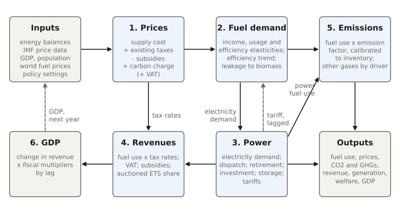
The module runs as a chain, with feedbacks that are always lagged. Figure 1 shows the order of calculation in a year. Prices are computed first for all years, because they depend on policy and world prices but not on quantities. Then, each year, fuel demand, power, revenue and emissions follow. Two quantities feed back, each with a one-year lag: revenue raised in year \(t\) moves output in year \(t+1\), and electricity demand in year \(t\) responds to last year’s tariff. Neither lag is an economic claim; both keep the spreadsheet free of circular references.
4 Data and baseline
The baseline starts from the country’s energy balance in the base year. Base-year fuel use by sector and fuel comes from the energy balance, mapped to CPAT’s fuels and sectors (CPAT Team 2024, Appendix B). The fuels are coal, natural gas, gasoline, diesel, liquefied petroleum gas (LPG), kerosene, jet fuel, other oil products, biomass and biofuels, renewables and electricity. The sectors fall into five groups: transport, buildings (residential, services, agriculture), industry, other energy use (mostly military) and power. Fuel transformation outside power, measured as primary less final energy use, is treated as one more industrial sector. Excel-AI uses 16 end-use subsectors plus power, with 2022 as the base year for fuel use and price data through 2024 (CPAT-AI Project 2026b); the 2023 edition of the documentation calibrates emissions to 2019 (CPAT Team 2024).
Output drives the baseline, and prices drive the policy. Real GDP and population come from the IMF World Economic Outlook, extended past its horizon by fixed rules; world fuel prices come from an average of IMF and World Bank forecasts by default (CPAT Team 2024; CPAT-AI Project 2026b, M0.1). In the baseline, fuel use grows with total real GDP through income elasticities, falls with an autonomous efficiency trend, and responds to whatever price changes the world-price forecasts and existing policies imply. Under the policy, the only new driver is the retail price, plus the effect of the policy’s revenue on output a year later.
Calibration fixes the starting point, not the response. Three calibrations keep the first projected years on track. Energy CO\(_2\) is scaled to the national inventory in the base year, so base-year emissions match (see the section on emissions, revenue and GDP). A demand shock adjusts fuel use in years of anomalous outturn: the documentation calibrates 2020 and 2021 to emissions outturns during COVID-19, and Excel-AI carries a switchable shock for 2023–2024 (CPAT Team 2024; CPAT-AI Project 2026b). In the power model, an implicit cost on coal is fitted so that the model reproduces the observed coal share of generation (see the power-sector section). None of these touches an elasticity, so none changes how the model responds to a carbon price.
5 Price formation
Every retail price is supply cost plus taxes, less subsidies. For sector group \(g\) (residential, industry, transport, power) and fuel \(f\), the documentation writes the retail price as
\[ p_{gf} = sp_{gf} + vat_{gf} + txo_{gf}, \tag{1}\]
where \(sp\) is the supply price, \(vat\) the VAT payment and \(txo\) excise and all other taxes net of consumer subsidies (CPAT Team 2024). In the historical years every component comes from the IMF’s fossil-fuel price and subsidy data (Black, Liu, et al. 2023), which give supply cost, producer subsidies, VAT, excises, consumer subsidies and the retail price by country, sector group and fuel. Excel-AI keeps existing and new carbon prices outside \(txo\), so that the after-tax price (equation 5) shows each instrument separately (CPAT-AI Project 2026b).
The supply price moves with world prices through its floating part. After the last historical year \(L\), the supply price is a fixed margin plus a part that follows the world price \(gp\) of the fuel’s commodity (crude oil, coal, the country’s gas market):
\[ sp_t = fixsp + \left(sp_{t-1} - fixsp - ps_{t-1}\right)\frac{gp_t}{gp_{t-1}} + ps_t, \tag{2}\]
where \(fixsp\) is the margin over world prices (plus the domestic production cost for coal and gas) and \(ps\) the producer subsidy per unit, negative where the subsidy lowers the price (CPAT-AI Project 2026b, M2.1, A2.5). The 2023 documentation states the subsidy’s sign two ways (documentation error DOC9); the corrected edition uses this convention throughout. Biomass has no world price and stays flat in real terms. All values are in real US dollars of a results year: domestic prices are deflated by the US consumer price index, world prices by the US GDP deflator. The legacy workbook added the margin and production cost in nominal dollars to real prices (legacy bug L172); the corrected method converts them first.
Price controls decide how much of a world-price change consumers see. Many countries regulate fuel prices, so a rise in the supply price is partly absorbed by a falling tax or a growing subsidy. CPAT captures this with a pass-through coefficient \(pcc\), read from the price data and bucketed into 0, 0.5 or 1:
\[ txo_t = txo_{t-1} - \left(sp_t - sp_{t-1}\right)\left(1 - pcc\right). \tag{3}\]
With \(pcc = 1\) the market is liberalized and every change in supply cost reaches the retail price; with \(pcc = 0\) a floating tax or subsidy absorbs the change (CPAT-AI Project 2026b, M2.2). A floor then makes the rule asymmetric: a positive existing tax never falls below its last historical level (CPAT-AI Project 2026b, A2.1). So under full price control a fuel that is subsidized keeps its retail price whatever happens to world prices, while a fuel that is taxed absorbs falls in world prices but passes rises through once its tax is back at its historical level. Legacy CPAT applied \((1 - pcc)\) twice in the first projected year (legacy bug L14); the corrected method applies it once.
VAT is levied on supply cost and taxes, and on the new carbon charge. The retail price before new policies is
\[ p^0_{gf} = \left(sp_{gf} + txo_{gf}\right)\left(1 + vatrate_{gf}\right). \tag{4}\]
Firms reclaim VAT, so where the price data leave the VAT rate blank Excel-AI applies the country’s general VAT rate to residential coal and gas and to oil products (scaled by the household share of each oil product), and a zero rate to power, industry and biomass (legacy bug L170, data issue I97) (CPAT-AI Project 2026c). This choice matters for revenue: a carbon charge on household gasoline raises VAT revenue as well as carbon revenue.
A carbon price enters as a charge per unit of energy, scaled by the emission factor and coverage. The national carbon tax \(NCT_t\) (US dollars per tonne of CO\(_2\)) follows a linear path from a start year to a target. For sector \(s\) and fuel \(f\) the charge per gigajoule is \(nct_{sf} = NCT_s\, ef_{sf}\, \varphi_{sf}\, x_{sf}\), where \(ef\) is the calibrated CO\(_2\) emission factor, \(\varphi\) the coverage and \(x\) an exemption factor that the user can phase out (CPAT-AI Project 2026b, M1.2–3, M2.4). The new ETS cost and any new excise are built the same way. The after-tax price by sector is then
\[ p_{sf} = \max\Big(p^0_{g(s)f} + \big(nct_{sf} + netsp_{sf} + nexc_{sf} + \Delta xcp_{sf}\big)\big(1 + vatrate_{g(s)f}\big),\ \underline{p}\Big), \tag{5}\]
where \(netsp\) is the ETS cost per unit, \(nexc\) the new excise, \(\Delta xcp\) the change in existing carbon pricing against the level already embedded in the price data, and \(\underline{p}\) a floor of 0.01 US dollars per gigajoule (CPAT-AI Project 2026b, M2.5). New policies pass through in full: CPAT assumes perfectly elastic fuel supply at the national level, so the whole charge falls on users.
Existing carbon prices count only as changes, so history is not counted twice. The IMF retail prices already contain whatever carbon tax or ETS price a country had in the data years. Excel-AI therefore adds only the change in existing carbon pricing, \(\Delta xcp\), against the embedded level; switching an existing scheme off lowers the price by its embedded level, and growth in an existing price raises it (CPAT-AI Project 2026b, A2.2). Existing schemes come from the World Bank’s carbon pricing dashboard (CPAT Team 2024, Appendix G).
An ETS is a carbon tax with a discount and a free-allocation split. CPAT treats a fully auctioned, frictionless ETS as equivalent to a carbon tax at its permit price (CPAT Team 2024). In practice the user sets a price, which Excel-AI converts to a tax-equivalent price by a volatility adjustment (1/1.1 at the default “medium” setting, replacing a hardcoded 1.1 in legacy, bug L15); a cap can also be imposed, and the model then solves for the price (CPAT-AI Project 2026b, A1.1). The share of allowances allocated free, \(\omega_s\), does not raise the user’s price; it moves into the shadow price that acts only on the efficiency margin (equation 6), which is how CPAT represents output-based allocation (CPAT-AI Project 2026b, M1.3–4). Revenue counts only the auctioned share.
Subsidy reform enters as separate wedges on the price. The user can phase out producer subsidies, consumer subsidies and price controls over a chosen period. Excel-AI adds each reform as its own wedge to the after-tax price, by fuel and sector, rather than mixing it into the pre-policy build-up; the price-control reform removes the floating part of \(txo\) in equation 3, as the CPAT-AI equation list sets out (CPAT-AI Project 2026b, M1.7). This keeps the baseline price untouched and makes the revenue from each reform visible.
Non-price policies are converted into shadow prices on the efficiency margin. Feebates, efficiency regulations and vehicle fuel-economy standards do not change what users pay per unit, but they change the efficiency of what they buy. CPAT converts each into a shadow carbon price \(\Sigma_s\), translated per unit of energy as \(sh_{sf} = \Sigma_s\, ef_{sf}\), which enters only the efficiency term of the demand equation (Black, Parry, et al. 2023; CPAT-AI Project 2026b, M1.4, M2.6). It raises no revenue. In legacy CPAT the regulation shadow price was computed but never applied (legacy bug L87); in the corrected method it acts. The documentation itself calls the semantics of this shadow price, with its 70 percent effectiveness weighting, “highly unclear” (CPAT Team 2024), and the issue remains open.
The Total Effective Carbon Price is a by-product of the price block. Because every component of the retail price is explicit, CPAT can report the total price signal on carbon, net of subsidies and including fuel excises, by fuel, sector and nationally (CPAT Team 2024). Paper 6.1 develops this into the Total Effective Carbon Price, the uniform carbon tax that would cut emissions by as much as a given policy mix (Stretton 2026d).
6 Demand response
One equation governs fuel use in every sector outside power. For sector \(s\) and fuel \(f\), fuel use \(F\) in year \(t\) relative to the year before is
\[ \frac{F_{sf,t}}{F_{sf,t-1}} = \underbrace{\left(\frac{1}{1 + \alpha_{sf} + \alpha^{+}_{s,t}}\right)^{1 + \epsilon_{U}}}_{\text{efficiency trend}} \Psi_t \underbrace{\left(\frac{Y_t}{Y_{t-1}}\right)^{\epsilon_{Y} inc_t}}_{\text{income}} \underbrace{\left(\frac{p_{sf,t}}{p_{sf,t-1}}\right)^{\epsilon_{U}}}_{\text{usage}} \underbrace{\left(\frac{p_{sf,t} + sh_{sf,t}}{p_{sf,t-1} + sh_{sf,t-1}}\right)^{\epsilon_{F}(1 + \epsilon_{U})}}_{\text{efficiency}}, \tag{6}\]
where \(\alpha\) is the autonomous efficiency improvement, \(\alpha^+\) any additional efficiency gain the user assigns to a policy (zero by default), \(\Psi_t\) a demand shock (1 in normal years), \(Y\) total real GDP, \(\epsilon_Y\) the income elasticity, \(inc_t\) an income-level adjustment, \(\epsilon_U\) the usage elasticity, \(\epsilon_F\) the efficiency elasticity and \(sh\) the shadow price of non-price policies (CPAT Team 2024; CPAT-AI Project 2026b, M3.1). The elasticities vary by country income group, sector and fuel. The form comes from the IMF tool (International Monetary Fund 2019; Black, Parry, et al. 2023).
The price response has two margins, and the second is damped by rebound. The usage margin is how much an existing car, boiler or furnace is used; the efficiency margin is how efficient the stock becomes. A permanent proportional price change \(\Delta \ln p\) with no shadow price changes fuel use by
\[ \Delta \ln F = \left(\epsilon_U + \epsilon_F + \epsilon_U \epsilon_F\right)\Delta \ln p. \tag{7}\]
The cross term \(\epsilon_U\epsilon_F\) is positive, because both elasticities are negative: a more efficient car is cheaper to drive, so it is driven more. With \(\epsilon_U = \epsilon_F = -0.3\), the total elasticity is \(-0.51\) rather than \(-0.6\), so the cross term gives back 15 percent of the gross response. The documentation compares this with the long-run rebound of 26–29 percent found for road transport in a meta-analysis of 74 studies (Dimitropoulos et al. 2018; CPAT Team 2024), but the comparison is loose: the meta-analysis measures how driving responds to fuel efficiency or to fuel cost per kilometre, not this cross term. A shadow price raises the efficiency margin only, through \(sh\) in the last term of equation 6, which is why a feebate cuts fuel use without raising the price paid per unit.
All elasticities are long-run, and the response is immediate. CPAT once had separate short- and long-run price elasticities; the team removed them “as the goal is not a short-term prediction but medium-term accuracy and simplicity” (CPAT Team 2024). equation 6 is applied year by year to the ratio of this year’s price to last year’s, so a permanent price step produces its full long-run response in the year it happens, and no further change after; Black, Parry, et al. (2023) state the same assumption, that the effects of prices on energy use are fully realized within one year. There is no partial adjustment toward a target (issue I62 in the CPAT-AI register). For phased policies, which is how carbon prices are usually introduced, the error is modest; for a sudden price jump the model overstates the first-year response.
Price elasticities are calibrated to a meta-analysis and adjusted for development. The starting point is the meta-analysis of energy price elasticities by Labandeira et al. (2017), which the documentation describes as about 2,000 estimates from 430 studies across seven fuels and four sectors. The CPAT team estimated target elasticities by fuel and sector from it, raised them slightly for developing countries, where the meta-analysis finds somewhat larger responses, and rounded usage and efficiency elasticities so that their emissions-weighted totals land within about 10 percent of the targets (CPAT Team 2024; World Bank and International Monetary Fund 2022). In the legacy elasticity table, usage elasticities run from \(-0.1\) to \(-0.7\) and efficiency elasticities from \(-0.2\) to \(-1.2\); low-, lower-middle- and upper-middle-income countries share one set of values, and high-income countries take usage elasticities 0.1 smaller in absolute value (CPAT-AI Project 2026b). Paper 5.4 checks these values against the wider evidence (Stretton 2026b), and Paper 6.1 sets them in a nested constant-elasticity-of-substitution (CES) demand system with explicit fuel switching (Stretton 2026d).
Income elasticities follow a hump in income per capita. Base income elasticities by sector come from Burke and Csereklyei (2016), whose estimates for 132 countries from 1960 to 2010 give an aggregate energy-GDP elasticity of 0.74; fuel-specific values are chosen so that the weighted average stays within one standard deviation of the sectoral estimates (CPAT Team 2024). Each is then scaled by a factor of income per capita that the CPAT team inferred from Gertler et al. (2016), who show that household purchases of energy-using assets rise nonlinearly with income: elasticities rise as households buy their first refrigerators, air conditioners and vehicles, peak around lower-middle income (about 3,000 US dollars per capita in the documentation’s figure) and decline toward the high-income level. That factor is \(inc_t\) in equation 6. Legacy CPAT applied it twice in the power model and anchored it to 2023 (legacy bug L3); the corrected method applies it once (CPAT-AI Project 2026c).
Total GDP, not GDP per capita, is the income driver. CPAT does not separate population growth from income growth: both enter through total GDP with the same income elasticity (CPAT Team 2024). A country whose GDP grows because its population grows therefore gets the income elasticity of a country getting richer. This is tracked as issue I71; separating the two would need a population elasticity near one and a per-capita income elasticity on the remainder.
The efficiency trend is half to one percent a year, and it rebounds too. The autonomous efficiency improvement \(\alpha\) is 0.5 or 1 percent a year depending on the fuel and sector (CPAT Team 2024). Because it enters with the exponent \(1 + \epsilon_U\), part of each efficiency gain is taken back in extra use; the documentation puts this exogenous rebound at 20 to 60 percent across fuels and sectors. The documentation also concedes that the trend mixes efficiency with shifting tastes (toward larger vehicles, for example) and “is not backed by detailed research”.
A worked example shows where a carbon price bites. Table 1 applies equation 7 to a carbon price of 50 US dollars per tonne of CO\(_2\), with stylized pre-policy prices, the default emission factors of the Intergovernmental Panel on Climate Change (Intergovernmental Panel on Climate Change 2006) and the legacy default elasticities for low- and middle-income countries. The carbon charge more than doubles the price of industrial coal, because coal is cheap per unit of energy and carbon-intensive, and cuts its use by about a third. The same carbon price adds about 13 percent to the price of diesel and 10 percent to gasoline, because road fuels already carry high taxes, and cuts their use by about 6 percent. Coal therefore shows by far the largest percentage cut; how many tonnes each fuel contributes depends on each country’s fuel mix. The cross term gives back 15 to 25 percent of the gross response.
2.Source/worked_examples.py).
| Fuel and sector | Price before (USD/GJ) | Carbon charge (USD/GJ) | Price change (%) | Total elasticity | Fuel use change (%) | Rebound (% of gross response) |
|---|---|---|---|---|---|---|
| Coal, industry | 4.0 | 4.73 | +118 | −0.58 | −36.4 | 17 |
| Natural gas, industry | 8.0 | 2.80 | +35 | −0.75 | −20.2 | 25 |
| Diesel, road transport | 27.7 | 3.71 | +13 | −0.51 | −6.2 | 15 |
| Gasoline, road transport | 33.6 | 3.46 | +10 | −0.64 | −6.1 | 20 |
Fuel switching is represented by separate margins, not by a substitution system. equation 6 has own-price elasticities only, so a carbon price that raises coal more than gas cuts coal more than gas, but does not by itself move demand from coal to gas. CPAT handles switching in four narrower ways. In power, the engineering model switches generation and investment between technologies on cost (see the power-sector section). In residential cooking, an optional leakage term moves households from the most-used modern cooking fuel to biomass when its price rises, with a substitution elasticity of 0.25 scaled by the stove efficiencies the documentation takes from Malla and Timilsina (2014), 0.58 (gas), 0.56 (LPG), 0.45 (kerosene) and 0.20 (biomass); in the documentation’s example a 10 percent rise in the gas price shifts about 0.9 percent of gas use to biomass (CPAT Team 2024). The leakage term is off by default in Excel-AI. In road transport, blended biofuels follow the fossil fuel they are blended with, and an optional engineering road model chooses between internal-combustion and electric vehicles by a logit on total cost of ownership (CPAT-AI Project 2026b, M5.2, A3.3). Self-generated renewables in buildings and industry follow equation 6 with the solar price. A full set of cross-price elasticities is absent; Paper 6.1 shows what a nested CES system adds (Stretton 2026d).
7 The power sector
CPAT has two power models, and the rebuilt version keeps the engineering one. The elasticity-based model, inherited from the IMF tool, projects total power demand with equation 6 and then shifts generation shares between technologies with conditional own-price elasticities of generation with respect to generation cost (International Monetary Fund 2019; CPAT Team 2024). It is simple but responds only to relative cost changes, has no capital stock, and can move generation faster than plants could be built. The techno-economic or “engineer” model, developed with the World Bank’s energy practice, tracks capacity by technology through investment and retirement and dispatches it each year. The documentation recommends “the average of the two models” for off-the-shelf use and the engineer model “for more tailored use” (CPAT Team 2024). Excel-AI builds only the engineer model, and this section describes it (CPAT-AI Project 2026b).
Four cost concepts serve four decisions. Dispatch uses the current variable cost: variable operation and maintenance, fuel cost and any carbon charge,
\[ vc_{f,t} = vop_f + \frac{\bar{p}_{f,t}}{\nu_f} + ip_{f,t} + ncp_{f,t}, \tag{8}\]
where \(\bar{p}\) is the fuel price averaged over the five years to \(t\), \(\nu\) the thermal efficiency, \(ip\) the implicit cost of coal and \(ncp\) the new policy cost per kilowatt-hour (CPAT-AI Project 2026b, M4.3). Investment uses a forward-looking levelized cost \(tic_f\): the discounted average of future variable costs, with full foresight of the announced carbon price, plus levelized capital, decommissioning, fixed operation and maintenance, transmission and the marginal cost of storage. The running cost of the system uses a cost-recovery generation cost that amortizes the capital of the existing stock. End-user tariffs use observed prices adjusted for changes in that cost (CPAT Team 2024). Legacy CPAT averaged the fuel price over two years before and two after the current year, so it read the future; the corrected method uses a trailing average (legacy bug L126). The 2023 documentation’s equation for the levelized cost writes the discount factor and the sum wrongly (DOC3).
The cost of capital is country- and technology-specific in the model, and income-based in the documentation. The 2023 documentation describes a default cost of capital by income group, 7.5 percent in high-income, 10 in upper-middle-income, 12.5 in lower-middle-income and 15 in low-income countries, following Steffen (2020)’s estimates of about 7.5 percent in OECD and 10 percent in non-OECD countries (CPAT Team 2024). The legacy workbook’s setting, which Excel-AI follows, is a country cost of capital from the workbook’s cost-of-capital table (7.5 percent where a country is missing) plus a technology premium by income group; the income-group rates are an option (CPAT-AI Project 2026b). The difference matters for capital-intensive renewables, whose levelized cost rises with the cost of capital more than that of fossil plants.
Electricity demand follows the fuel equation, with last year’s tariff. Power demand in each of four demand groups (transport, residential, industry, services) follows equation 6, with electricity elasticities and a blend of last year’s residential and industrial tariffs (CPAT-AI Project 2026b, M4.1). Using last year’s price avoids a circular reference: this year’s tariff depends on this year’s generation mix, which depends on demand. Required generation adds net exports, transmission losses and the energy sector’s own use in their base-year proportions. Two legacy bugs changed demand here: services demand grew with the industrial multiple after 2023 (L1), and the efficiency trend used the efficiency elasticity instead of the usage elasticity in its rebound exponent (L2). Both are fixed.
Dispatch runs renewables and nuclear first and splits the rest between coal and gas by a logit. Wind, solar, hydro, other renewables, nuclear, oil and biomass generate at their capacity factors. Coal and gas cover the remainder: each first supplies the minimum it must, given the other’s maximum output at a capacity factor of 0.9, and the rest is shared by
\[ \lambda_f = \frac{e^{-K_{d} H_f}}{\sum_{f'} e^{-K_{d} H_{f'}}}, \qquad H_f = \frac{vc_f}{\min_{f'} vc_{f'}}, \qquad f, f' \in \{\text{coal}, \text{gas}\}, \tag{9}\]
with \(K_d = 2\) by default (CPAT Team 2024; CPAT-AI Project 2026b, M4.4). Plants under power purchase agreements can be set to run at their capacity factor whatever their cost. The logit stands in for the hourly merit order, regional constraints and plant heterogeneity that a one-period annual model cannot represent: it makes the cheaper fuel dominate without taking everything.
Capacity follows a stock-flow identity with three kinds of retirement. Capacity by technology is
\[ cap_{f,t} = cap_{f,t-1} - ret_{f,t-1} + inv_{f,t-1}, \qquad ret_{f,t} = \frac{cap_{f,t}}{lif_f}, \tag{10}\]
so plants retire at the reciprocal of their lifetime unless plant-level data give a schedule, as a plant-level tracker does for coal (CPAT Team 2024; CPAT-AI Project 2026b, M4.5). On top of scheduled retirement, coal can retire early when its variable cost, including the carbon charge, exceeds the full cost of wind and solar: a logit on those costs sets the share of the maximum early retirement (80 percent of coal’s effective capacity by default) that happens, limited by how fast wind and solar can grow (CPAT-AI Project 2026b). The 2023 documentation writes equation 10 in generation and sums it over fuels (DOC11); it is capacity, by technology.
Investment is allocated by a logit on levelized cost, within scale-up limits. The capacity needed is required generation less the effective capacity left after retirement, and capacity built in year \(t\) comes online in \(t+1\). Legacy CPAT sized new capacity for this year’s demand although it arrives next year (legacy bug L67); the corrected method sizes it for next year’s estimated requirement. The need is shared among permitted technologies by
\[ \frac{ivp_{f,t}}{\sum_{f'} ivp_{f',t}} = \zeta_f \frac{e^{-K_i H_{i,f}}}{\sum_{f'} \zeta_{f'} e^{-K_i H_{i,f'}}}, \qquad H_{i,f} = \frac{tic_f}{\min_{f':\,\zeta_{f'} = 1} tic_{f'}}, \tag{11}\]
with \(K_i = 2\) and \(\zeta_f\) equal to 1 for permitted technologies and 0 otherwise (CPAT Team 2024; CPAT-AI Project 2026b, M4.6). The documentation says the two curvature parameters are “set subjectively at 2 for both dispatch and investment, which we believe produces realistic results”. By default a technology is permitted if it already has capacity; hydro and nuclear are better set as exogenous plans, because CPAT has no resource curves. Each technology’s additions are capped at a share of total effective capacity (capacity times capacity factor) a year: for wind and solar, 2 percentage points each in most countries, with higher country-specific values for China and India in the current data; 5 for coal, gas and hydro; and 2 for the others (CPAT Team 2024; CPAT-AI Project 2026b). A second round gives any unplaced need to the cheapest technologies with room under their caps. Legacy CPAT divided each technology’s cost by the cheapest technology even when that technology was not permitted to be built (legacy bug L6); the corrected method divides by the cheapest permitted one.
The cost of integrating renewables is a storage charge that rises with their share. CPAT has no hourly load curve, so it charges variable renewables for the storage a high share would need. Short-term storage, in hours of battery per unit of average generation, is \(sst = 9v^2\), where \(v\) is the share of wind, solar and other non-hydro renewables in generation, the documentation’s rounded fit to the global system modeling of Bogdanov et al. (2019). The marginal requirement is \(d\,sst/dv = 18v\); the 2023 documentation prints \(18v^2\) (DOC6). Long-term storage, priced as electrolyzer capacity, is zero below a 75 percent share and rises quadratically to 1 at 100 percent, with one-third of its cost allocated to power (CPAT Team 2024). The levelized cost of the marginal storage is added to the investment cost of variable renewables, so their storage-inclusive cost can rise as their share grows even while panel and turbine costs fall. Legacy CPAT applied the one-third allocation twice (legacy bug L4); the corrected method applies it once (CPAT-AI Project 2026c).
An implicit cost on coal calibrates the model to the observed coal share. With costs alone, the model tends to overstate coal’s share of generation, because it omits environmental regulation, the inflexibility of coal plants and the value of gas for balancing. CPAT adds a positive implicit price on coal, fitted by goal seek so that the modeled coal share matches the observed share, for 85 countries where it is needed (CPAT Team 2024; CPAT-AI Project 2026b). It acts like a pre-existing, unpriced coal penalty: it lowers baseline coal use and so the carbon price’s room to cut it.
Tariffs pass changes in generation cost and the carbon charge through to users. Observed residential and industrial prices are the starting point. After the last historical year, the price before new policies changes by the pass-through times the change in the supply cost (last year’s generation-weighted average cost plus transmission of 40 US dollars per megawatt-hour for households and 15 for industry), plus VAT; the new policy cost per kilowatt-hour, weighted by generation shares, is then added with VAT (CPAT-AI Project 2026b, M4.7). Under output-based rebating the carbon cost stays in dispatch and investment but is returned to users, so tariffs do not rise. The documentation instead adds a markup calibrated to historical prices and, in its 2023 edition, prints it with the wrong sign (DOC2); with the sign corrected, both methods start from the observed tariff and pass cost changes through.
State-owned utilities are assumed to respond to the carbon price as a shadow price. Where generation is planned by a state utility, CPAT assumes the plan uses the carbon price as a shadow price in investment appraisal, so the investment response is the same as in a private market (CPAT Team 2024). That is generous to carbon pricing in countries where the utility answers to a ministry rather than to prices. The documentation flags it as an issue and suggests making the investment decision explicit, which would show what a finance ministry needs to tell its utilities to do.
8 A proposed alternative: penalty-based investment allocation
This section describes a proposal, not CPAT. The investment logit in equation 11 works, but it has two features a finance ministry finds hard to explain. It never gives a technology a zero share: in a stylized case with oil-fired power at 120 US dollars per megawatt-hour against solar at 45, the logit still gives oil 1.4 percent of new investment (Table 2). And it depends on cost ratios, not differences, so adding the same carbon charge to every technology changes their shares. A background note by the author proposed replacing it with allocation rules derived from a quadratic penalty. This section restates that proposal against the right benchmark, corrects one step of it, and labels it as a proposed alternative to logit share rules, not part of any CPAT version.
The CPAT logit is itself a penalized cost minimum, with a penalty weight in dollars. Let \(C_i\) be the levelized cost of technology \(i\) and \(s_i\) its share of new investment. The share vector that minimizes expected cost plus an entropy penalty on concentration,
\[ \min_{s} \sum_{i=1}^{N} \left(C_i s_i + \tau\, s_i \ln s_i\right) \quad \text{s.t.} \quad \sum_i s_i = 1, \tag{12}\]
is the logit \(s_i = e^{-C_i/\tau}/\sum_j e^{-C_j/\tau}\) (Appendix B). This is the representative-consumer reading of the logit, in which variety-seeking is an entropy term in a deterministic objective (Anderson et al. 1988). CPAT’s rule is the case \(\tau = C_{min}/K\). So \(K = 2\) has an economic meaning after all: with solar at 45 dollars per megawatt-hour the cheapest option, the planner behaves as if concentration cost an entropy penalty with a weight of 22.5 dollars per megawatt-hour. Two features follow. The penalty’s marginal cost, \(\tau(1 + \ln s_i)\), falls without limit as a share approaches zero, so no technology ever drops out. And the weight moves with the cheapest cost: a charge that raised every technology’s cost by the same amount would raise \(\tau\) and flatten the shares, although no cost difference had changed. This is the ratio form seen as a penalty.
The velocity rule replaces the entropy penalty with a quadratic one. The planner chooses shares to minimize cost plus a quadratic penalty on concentration,
\[ \min_{s} \sum_{i=1}^{N} \left(C_i s_i + \frac{\lambda}{2} s_i^2\right) \quad \text{s.t.} \quad \sum_i s_i = 1,\ s_i \ge 0, \tag{13}\]
where \(\lambda\), in dollars per megawatt-hour, measures the diversification pressure: integration costs, risk spreading and pipeline limits that rise as one technology dominates. At an interior solution the first-order condition \(C_i + \lambda s_i = \mu\) gives
\[ s_i = \frac{1}{N} + \frac{\bar{C} - C_i}{\lambda}, \qquad \bar{C} = \frac{1}{N}\sum_i C_i. \tag{14}\]
Shares are linear in cost differences. A technology 10 dollars per megawatt-hour cheaper than average gets \(10/\lambda\) more of the market. As \(\lambda \to 0\) the rule tends to least cost; as \(\lambda \to \infty\), to equal shares. The term \(C_i + \lambda s_i\) has a natural reading as a “systemic” levelized cost, the plant’s own cost plus the system cost of adding more of the same. Because the penalty’s marginal cost at a zero share is finite, a technology whose cost exceeds the others’ systemic cost gets nothing. The solution of equation 13 is the Euclidean projection of \(-C/\lambda\) onto the set of shares, the operation known in machine learning as sparsemax, introduced there as a sparse alternative to the logit (Martins and Astudillo 2016).
Uncompetitive technologies drop out exactly, if the active set is recomputed. Where equation 14 gives a negative share, the constraint \(s_i \ge 0\) binds and the technology gets nothing. The correct solution then recomputes the mean cost over the technologies that remain and applies equation 14 again with \(N\) equal to their number, repeating until no share is negative. This is the exact minimizer of equation 13. The background note instead rescales the positive shares in proportion so they sum to one, which is not the minimizer: in its own five-technology example with costs of 20, 30, 40, 50 and 100 US dollars per megawatt-hour and \(\lambda = 100\), proportional rescaling gives 36.4, 28.8, 21.2 and 13.6 percent to the first four, where the minimizer gives 40, 30, 20 and 10 percent (2.Source/worked_examples.py). Any implementation should use the active-set rule.
The acceleration rule penalizes changes in shares instead of their level. Investment pipelines, procurement rules and politics limit how fast the mix can move. Replacing the level penalty with a penalty on the change from last year, \(\frac{\lambda_a}{2}(s_{i,t} - s_{i,t-1})^2\), gives the update rule
\[ s_{i,t} = s_{i,t-1} + \frac{\bar{C}_t - C_{i,t}}{\lambda_a}, \tag{15}\]
so a technology cheaper than average gains share at a speed set by \(\lambda_a\). In continuous time this is \(\lambda_a\, ds_i/dt = \bar{C} - C_i\), a linear counterpart of the logistic share equations of FTT:Power (Mercure 2012). equation 15 has no interior steady state unless all costs are equal; it describes a path, not a destination. It is the penalized form of CPAT’s scale-up caps: a cap is a penalty that is zero up to a limit and infinite beyond it, while equation 15 charges the speed of change continuously.
Combining the two gives a target and a speed. With both penalties and a set of system-cost adjustments \(C^{sys}_{i,t}\) evaluated at last year’s shares, the first-order condition gives
\[ s_{i,t} = \frac{\lambda_a s_{i,t-1} + \lambda_v/N}{\lambda_v + \lambda_a} + \frac{\bar{C}^{e}_t - C^{e}_{i,t}}{\lambda_v + \lambda_a}, \qquad C^{e}_{i,t} = C_{i,t} + C^{sys}_{i,t}, \tag{16}\]
where \(\bar{C}^e\) is the mean effective cost (Appendix B). The first term is a weighted average of last year’s share and the equal share; the second is the cost signal. The note proposes system terms of three kinds: a flexibility benefit for gas that rises with the gas share, an integration cost for variable renewables that rises with their combined share (the role CPAT’s storage charge plays now), and a land-footprint cost that falls with population density.
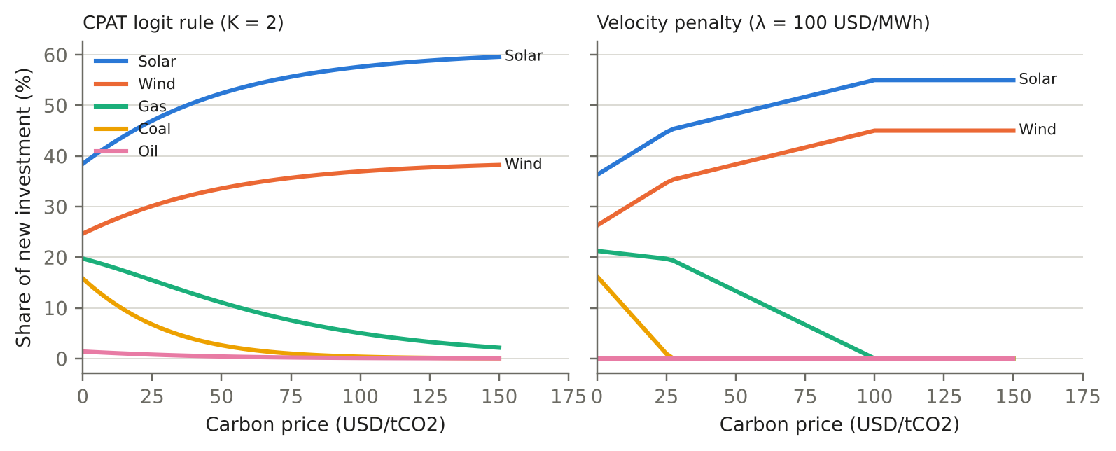
The two rules respond differently to a carbon price. Table 2 and Figure 2 compare the logit rule (equation 11) with the velocity rule (equation 14) for five stylized technologies as a carbon price rises. At zero carbon price they give similar shares, except that the velocity rule gives oil nothing. At 75 dollars per tonne the velocity rule has already pushed coal to zero and gas to 6.7 percent; the logit keeps coal at 1.0 percent and gas at 7.5. At high carbon prices, once only solar and wind remain in play, the logit’s ratio form holds solar at about 61 percent however expensive fossil power becomes, because the solar-to-wind cost ratio is fixed, while the velocity rule settles at 55 percent solar and 45 percent wind, set by their 10-dollar cost difference and \(\lambda\). Neither is right in general; the difference is in the shape of the penalty, and both weights can be stated in dollars per megawatt-hour.
2.Source/worked_examples.py).
| Technology | Cost, no carbon price | Logit share (%) | Velocity share (%) | Cost at USD 75/tCO\(_2\) | Logit share (%) | Velocity share (%) |
|---|---|---|---|---|---|---|
| Solar | 45.0 | 38.4 | 36.2 | 45.0 | 55.6 | 51.7 |
| Wind | 55.0 | 24.6 | 26.2 | 55.0 | 35.7 | 41.7 |
| Gas | 60.0 | 19.7 | 21.2 | 90.0 | 7.5 | 6.7 |
| Coal | 65.0 | 15.8 | 16.2 | 136.2 | 1.0 | 0.0 |
| Oil | 120.0 | 1.4 | 0.0 | 172.5 | 0.2 | 0.0 |
2.Source/make_figures.py).
The proposal has costs a reviewer should weigh. Both rules depend on how the technology list is drawn. Under the exact active-set rule a technology that ends at zero has no effect on the others: adding a sixth technology at 300 dollars per megawatt-hour leaves every share in Table 2 unchanged. But listing one technology twice changes the result under either rule: splitting solar into two identical entries raises solar’s combined share at zero carbon price from 36.2 to 58.0 percent under the velocity rule and from 38.4 to 55.5 percent under the logit. Either rule needs a fixed, published technology list. The velocity rule is piecewise linear, so shares have kinks where a technology enters or leaves (visible in Figure 2). And \(\lambda\) still has to be calibrated, by fitting observed investment shares across countries and years or by stating the cost advantage that should buy a given share; the same is true of the logit’s \(\tau\), which CPAT has never estimated. The proposal is worth testing in CPAT Python as a switchable alternative before any change to the default; the switch would leave dispatch, retirement and the scale-up limits as they are.
9 Emissions, revenue and GDP
Energy CO\(_2\) is fuel use times a calibrated emission factor. For each sector and fuel, including the fuel input to power,
\[ em_{sf} = F_{sf}\, ef_{sf}, \qquad em_{CO_2} = \sum_s\sum_f em_{sf}, \tag{17}\]
with emission factors from the GAINS model of the International Institute for Applied Systems Analysis (IIASA) by country, sector and fuel, or global factors of the International Energy Agency as an option (CPAT Team 2024; CPAT-AI Project 2026b, M7.1). The GAINS factors include process emissions, so the module scales all energy CO\(_2\) by one factor so that base-year emissions equal the national inventory. Emissions are territorial: methane leaked upstream from imported gas counts in the producing country. The documentation calls the GAINS-plus-calibration approach “unsatisfactory” and suggests deriving weighted factors from detailed energy balances (CPAT Team 2024); the CPAT-AI register tracks the same factor data as an open data issue.
Other gases and sectors grow with simple drivers. Energy nitrous oxide scales with energy CO\(_2\); industrial process emissions grow with industrial energy CO\(_2\); agriculture with output and population through elasticities; waste with population; emissions from land use, land-use change and forestry in countries where that sector is a net source decline by 2.5 percent a year in both scenarios (CPAT Team 2024; CPAT-AI Project 2026b, M7.2). Methane from fossil fuel production is production times an emission factor, and a methane fee cuts the factor along an abatement curve \(red = A \cdot mf^{B}\). By default the carbon price also applies to the other greenhouse gases, so their emissions fall in proportion to fossil CO\(_2\); this can be switched off. Legacy CPAT held non-energy methane constant and never applied the computed abatement (legacy bug L18); the corrected method grows it with income and population and abates each source along its own curve (CPAT-AI Project 2026c).
Nationally determined contributions are converted to a 2030 emissions target for comparison. CPAT harmonizes the nationally determined contributions (NDCs) of 192 countries, whether expressed against business as usual, as a fixed level, against a historical year or as an intensity, into a 2030 level of greenhouse gases excluding land use and forestry, and reports the gap between it and the baseline and policy paths (CPAT Team 2024). Because the carbon price mainly cuts energy emissions, countries with large agriculture or land-use emissions face a high burden on energy to close the gap.
Revenue is fuel use times tax rates, compared between scenarios. Revenue from new policies, in each sector and fuel, is
\[ rev^{new}_{sf} = \theta F_{sf}\Big(nct_{sf} + nexc_{sf} + \rho\, netsp_{sf} + vatrate\,\big(nct_{sf} + netsp_{sf} + nexc_{sf}\big)\Big), \tag{18}\]
where \(\theta\) converts fuel use in kilotonnes of oil equivalent to gigajoules (41,868 gigajoules per kilotonne) and \(\rho\) is the auctioned share of ETS allowances (CPAT-AI Project 2026b, M6.1). Revenue from existing taxes is fuel use times existing excise and VAT; existing consumer subsidies are a negative revenue; producer subsidies and renewable subsidies are costs; power adds tariff VAT, the subsidy gap between tariff and modeled cost, and any rebate (CPAT-AI Project 2026b, M6.2–3). The policy’s fiscal effect is the difference in total revenue from the baseline. It therefore includes the base effect: a carbon tax shrinks the base of existing fuel excises, so its net revenue is less than the gross carbon revenue (CPAT Team 2024).
Output responds to the change in revenue, a year later, through fiscal multipliers. The fiscal impulse is the change in the revenue gain against the baseline, as a share of baseline GDP. Its effect on GDP sums, over the previous 20 years of impulses, the contractionary effect of the revenue raised (with the multiplier for energy taxes) and the expansionary effect of each use of the revenue the user chooses (labor tax cuts, corporate tax cuts, public investment, goods and services, transfers), each with its own multiplier by lag:
\[ \varepsilon^{GDP}_t = -\sum_{k=0}^{19} imp_{t-k}\, m_{exc}(k) + \sum_i sh_i \sum_{k=0}^{19} imp^{p}_{t-k}\, m_i(k), \qquad Y_t = Y^0_t\left(1 + \varepsilon^{GDP}_{t-1}\right), \tag{19}\]
where \(sh_i\) is the share of revenue given to use \(i\) and \(imp^p\) the impulse counted from the start year of carbon pricing (CPAT-AI Project 2026b, M8.1–3). The multipliers come from the World Bank’s macro-fiscal model, MFMod (Burns et al. 2019), from panel estimates, or from the user (CPAT Team 2024). The 2023 documentation describes the multipliers but gives no equation for how they enter the model (DOC1); the corrected edition adds the section that equation 19 summarizes (CPAT-AI Project 2026a). Legacy CPAT added the GDP effect to the GDP growth rate every year, so a one-off level effect compounded (legacy bug L24); the corrected method raises the level.
Welfare is accounted with Harberger triangles and valued co-benefits. The efficiency cost of a carbon charge in each fuel market is approximately half the charge times the fall in fuel use; where a prior tax exists, the prior tax times the fall in use is added, the trapezoid of standard tax analysis (CPAT Team 2024). The 2023 documentation’s equation for this cost uses the wrong symbol and describes the term wrongly (DOC8). Against it, CPAT sets the domestic benefits of lower fuel use: averted air pollution deaths and illness from the air pollution module, fewer road accidents and less congestion from the road transport module, and averted climate damage valued at a social cost of carbon (by default 75 US dollars per tonne in 2030, rising 4 percent a year in real terms, or the country-level values of Ricke et al. (2018)). The net is reported as a share of GDP.
10 Outputs, parameters and how to use them
The module’s outputs are what a budget memo needs. For each scenario and year it reports fuel use by sector and fuel, retail prices and price indices, CO\(_2\) and other greenhouse gases against the NDC target, revenue by instrument and as a share of GDP, generation and capacity by technology with investment spending, electricity tariffs, the efficiency cost and co-benefits, and GDP (CPAT Team 2024). It passes prices and quantities to the distribution module, which estimates the burden by household decile, and to the air pollution and road transport modules. The useful outputs are the differences from the baseline, read alongside the price changes that produced them.
A small set of parameters drives the results. Table 3 lists them with their defaults and sources. Three dominate. The usage and efficiency elasticities set the size of the demand response (Paper 5.4 tests them). The income elasticities and the efficiency trend set the baseline, and so the room for any policy to cut. And, in power, the scale-up limits on wind and solar often bind before costs do, so for large carbon prices the investment response is set by an assumption about build rates rather than by the price. The validation evidence for the module as a whole, including comparisons with IEA scenarios, Enerdata and the World Bank’s Electricity Planning Model and a hindcast, is the subject of Paper 5.3 (Stretton 2026f).
data/Public01/tidy/xai_elasticities.csv); other defaults are from the CPAT documentation and the CPAT-AI methods notes. “Judgment” means the documentation gives no empirical source. Source: CPAT Team (2024); CPAT-AI Project (2026b).
| Parameter | Default | Source |
|---|---|---|
| Usage price elasticity \(\epsilon_U\) | −0.1 to −0.7 by fuel and sector; 0.1 smaller in absolute value for high-income countries | Calibrated to Labandeira et al. (2017; CPAT Team 2024) |
| Efficiency price elasticity \(\epsilon_F\) | −0.2 to −1.2 by fuel and sector | Calibrated to Labandeira et al. (2017) |
| Income elasticity \(\epsilon_Y\) | 0 to 1.2 by fuel and sector, scaled by income per capita | Burke and Csereklyei (2016); inferred from Gertler et al. (2016) |
| Autonomous efficiency improvement \(\alpha\) | 0.5 or 1 percent a year | Documentation; “not backed by detailed research” (CPAT Team 2024) |
| Biomass leakage | Substitution elasticity 0.25; stove efficiencies 0.58 (gas), 0.56 (LPG), 0.45 (kerosene), 0.20 (biomass); off by default in Excel-AI | Malla and Timilsina (2014; CPAT Team 2024) |
| Pass-through of world prices \(pcc\) | 0, 0.5 or 1, bucketed from the price data; positive taxes floored at their last level | IMF price data (Black, Liu, et al. 2023; CPAT-AI Project 2026b) |
| ETS volatility adjustment | 1/1.1 at “medium” | CPAT default (CPAT-AI Project 2026b) |
| Logit curvature \(K\) (dispatch, investment) | 2 and 2 (“set subjectively”) | Judgment (CPAT Team 2024) |
| Cost of capital | Country rate plus a technology premium (model); 7.5, 10, 12.5, 15 percent by income group (documentation, an option in the model) | Steffen (2020; CPAT Team 2024; CPAT-AI Project 2026b) |
| Maximum annual additions | Wind and solar 2 percentage points of effective capacity each in most countries (higher for China and India); coal, gas, hydro 5; others 2 | CPAT default (CPAT Team 2024; CPAT-AI Project 2026b) |
| Maximum early coal retirement; maximum coal and gas capacity factor | 80 percent of coal’s effective capacity; 0.9 | CPAT default (CPAT-AI Project 2026b) |
| Short-term storage requirement | \(9v^2\) hours per unit of average generation | Rounded fit to Bogdanov et al. (2019) |
| Long-term storage | Zero below 75 percent variable renewables; one-third of cost allocated to power | CPAT default |
| Transmission and distribution adders | 40 (residential) and 15 (industry) USD/MWh | CPAT default (CPAT Team 2024; CPAT-AI Project 2026b) |
| Emission factors | GAINS by country, sector and fuel, calibrated to the inventory; IEA option | IIASA GAINS; national inventories |
| Land-use emissions trend, net-source countries | −2.5 percent a year | Documentation (CPAT Team 2024) |
| Social cost of carbon | 75 USD/tCO\(_2\) in 2030, +4 percent a year real; country values optional | CPAT default; Ricke et al. (2018) |
| Fiscal multipliers | By income group from MFMod, panel estimates, or user, by lag | Burns et al. (2019; CPAT Team 2024) |
Use the module for phased, medium-term reforms, and read it as a first estimate. The module is built for anticipated policies phased in over several years and assessed over a decade: a carbon price rising to a target, a subsidy phased out, an excise reformed. Used that way, its known biases are small relative to the uncertainty in the parameters. For a first engagement with a ministry, run the default, read the price changes before the quantity changes, check the base-year calibration against national data, and replace defaults (the power plan, the elasticities, the multipliers) with country evidence where it exists. For a sudden price shock, a short-run forecast or a power system dominated by hydro or a state utility, use a more detailed model alongside it, as the documentation itself advises (CPAT Team 2024).
11 Key limitations
The strongest objection is that a model this simple should not inform fiscal decisions. A sceptic would point to long-run elasticities that act within a year, own-price responses only, a fixed world and a power sector whose investment response rests on two judgment calls. The answer is threefold. The module is a first estimate for phased, medium-term reforms, where the omitted dynamics matter least. Its biases mostly have known signs, set out below, so a ministry can say which way a result is likely to be wrong. And its two central parameter sets are checked against evidence: the price elasticities against meta-analytic estimates (Paper 5.4, Stretton 2026b), and the module’s responses against other models and a back-cast (Paper 5.3, Stretton 2026f). What the module should not do is give a precise power-sector path under a large carbon price; there, the build-rate caps and the logit’s penalty weight set the answer, and a result should say so.
The demand system has no lags and almost no substitution. All elasticities are long-run and act in one year, so the model overstates first-year responses to price jumps (issue I62). Own-price elasticities dominate, so a carbon price that changes relative fuel prices does not move demand between fuels except in power, cooking and road vehicles. This understates switching from coal to gas in industry and overstates the fall in total energy use. Paper 6.1 shows how a nested CES system with partial adjustment fixes both (Stretton 2026d). Road transport has a further problem: CPAT describes road transport three times, in a simple fuel equation, an engineering fleet model and a co-benefits module that values congestion, accidents and road damage, and the three are not consistent: the co-benefits module always takes vehicle-kilometers from the fleet model, even when fuel use and emissions follow the fuel equation, so the change in driving it values need not match the modeled change in fuel use (Paper 6.4, Stretton 2026a; CPAT-AI Project 2026c, no. I100).
Population is treated as income, and the efficiency trend is a residual. Total GDP drives demand with one elasticity, so population growth gets the elasticity of rising income (issue I71). The autonomous efficiency trend is judgmental and mixes technical progress with changing tastes. Both mainly affect the baseline, and through it the level of emissions a policy cuts from, more than the percentage response.
The power model is annual and its allocation rules are not estimated. With one period a year, CPAT cannot represent the hourly match of supply and demand, reserve margins or renewable resource quality; the storage charge and the scale-up limits stand in for all three. The logit curvature is set by judgment, the coal implicit cost absorbs whatever the cost data miss, and state utilities are assumed to treat the carbon price as a shadow price. For deep decarbonization, a dedicated capacity-expansion model should check the result; the documentation states that CPAT “does not aim to replace models like EPM”, the World Bank’s Electricity Planning Model (CPAT Team 2024).
Prices are national, supply is flat and the world is fixed. CPAT assumes fuel supply is perfectly elastic at world prices, that the policy does not change world prices, and that nothing leaks across borders. A carbon price in a large economy or a coordinated global price would change world fuel prices; a carbon price without border adjustment would move some energy-intensive production abroad. Neither is in the module; the CBAM tool of Paper 6.2 (Stretton 2026e) addresses exposure to the European Union’s Carbon Border Adjustment Mechanism separately.
Non-price policies rest on a weak bridge. Regulations, standards and feebates enter as shadow prices on the efficiency margin with an effectiveness weight whose meaning the documentation itself calls unclear. Comparing a regulation with a carbon tax in CPAT is therefore only as good as that conversion. The policy-equivalent approach of Black et al. (2022) uses the same machinery and inherits the same weakness.
Data quality limits more than method does. The price data have blank VAT cells that may be missing values or true zeros; emission factors come as base and final values only; capacity by technology is estimated, not observed (CPAT-AI Project 2026c). Each tracked data issue is replicated in the rebuilt model until the data are fixed, so the results inherit them.
12 Conclusion
The CPAT mitigation module fits in fourteen equations: a price identity with a carbon charge, a constant-elasticity demand equation with two price margins, a power model with a logit dispatch, a stock-flow capacity identity and a logit investment rule, an emissions identity, a revenue identity and a lagged multiplier rule for output. Stated that way, its strengths are plain: every number can be traced to a price, a quantity and an elasticity, and every policy works through the price it changes. So are its weaknesses: no lags, little substitution, an annual power model whose investment response rests on judgment, and a fixed world.
Stating a model this briefly is a test of it. The documentation errors and legacy bugs in Appendix A were found by writing each equation once and checking it against a running model, and writing the investment rule as an optimization showed that its curvature parameter is a penalty weight in dollars per megawatt-hour that can be estimated and argued about. The next steps follow from the limitations: estimate that weight, or test the quadratic-penalty rule behind a switch; add partial adjustment and fuel switching along the lines of Paper 6.1; and extend the corrected model’s data from one country to all.
Downloads
References
13 Appendix A: Where the documentation and the corrected method differ
The CPAT-AI project keeps a register of every difference between the documentation, legacy CPAT and the rebuilt model (CPAT-AI Project 2026c). Table 4 lists those that change a method stated in this paper. “DOC” items are errors in the 2023 edition of the documentation that do not affect the model; each one listed here is corrected in the edition of 31 October 2026 (CPAT-AI Project 2026a). “L” items are bugs in the legacy workbook, fixed in Excel-AI and CPAT Python and never replicated. “I” items are issues, replicated and tracked.
| Code | Where | 2023 documentation or legacy workbook | Corrected method (this paper) |
|---|---|---|---|
| DOC1 | GDP | Multipliers described; no in-model equation | equation 19: impulse, multipliers by lag, GDP level a year later |
| DOC2 | Tariffs | Markup \(mu = gnc^{av} + tmc - hrp\) | \(mu = hrp - gnc^{av} - tmc\); Excel-AI passes cost changes through from observed prices |
| DOC3 | Levelized cost | Discount factor and levelized cost written wrongly | \(dfc_t = (1+wacc)^{-(t-t_0)}\); \(tic = \sum_t vc_t\, cf\, dfc_t / \sum_t cf\, dfc_t + fix^{fl}\) |
| DOC4 | Power demand | GDP elasticity \(\epsilon_G\) never defined | \(\epsilon_Y\) with the income adjustment, as in equation 6 |
| DOC6 | Storage | \(d\,sst/dv = 18v^2\) | \(d\,sst/dv = 18v\) |
| DOC8 | Welfare | Wrong symbol and description of the efficiency cost | Harberger trapezoid |
| DOC9 | Prices | Producer subsidy added in one place, subtracted in another | One sign convention, equation 2 |
| DOC11 | Capacity | Stock equation in generation, summed over fuels | equation 10, capacity by technology |
| L1, L2, L3 | Power demand | Services use industry multiple; efficiency trend rebounds with \(\epsilon_F\); income factor applied twice | Own multiple; \(\epsilon_U\); income factor once |
| L4 | Storage | Long-term storage allocation (one-third) applied twice | Applied once |
| L6 | Investment | Logit costs divided by the cheapest technology, permitted or not | Divided by the cheapest permitted technology, equation 11 |
| L14 | Prices | Pass-through applied twice in first projected year | Applied once, equation 3 |
| L15 | ETS | Hardcoded relative price of 1.1 | Volatility adjustment, 1/1.1 at “medium” |
| L18 | Methane | Non-energy methane constant; abatement not applied | Grows with drivers; abated along its own curve |
| L24 | GDP | Effect added to growth every year | Effect raises the level, equation 19 |
| L67 | Investment | New capacity sized for this year although online next year | Sized for next year |
| L87 | Regulations | Shadow price computed but never applied | Applied to the efficiency margin |
| L126 | Power costs | Fuel price averaged over two past and two future years | Trailing five-year average |
| L170 | Prices | Blank VAT cells read as a zero rate | General rate for household fuels, zero for firms |
| L172 | Prices | Margins added in nominal dollars to real prices | Converted to real first |
| I62, I71 | Demand | No partial adjustment; population takes the income elasticity | Replicated and tracked (see the section on limitations) |
14 Appendix B: Derivation of the allocation rules
Logit as an entropy-penalized minimum. The Lagrangian of equation 12 is \(\mathcal{L} = \sum_i (C_i s_i + \tau s_i \ln s_i) - \mu(\sum_i s_i - 1)\). The first-order condition \(C_i + \tau(1 + \ln s_i) = \mu\) gives \(s_i = e^{(\mu - \tau - C_i)/\tau}\), and the adding-up constraint gives \(s_i = e^{-C_i/\tau}/\sum_j e^{-C_j/\tau}\). The objective is strictly convex on the simplex and the entropy term’s derivative tends to \(-\infty\) as \(s_i \to 0\), so the minimizer is unique and interior. Setting \(\tau = C_{min}/K\) gives CPAT’s rule, \(s_i \propto e^{-K C_i / C_{min}}\).
Velocity rule. The Lagrangian of equation 13 is \(\mathcal{L} = \sum_i (C_i s_i + \tfrac{\lambda}{2}s_i^2) - \mu(\sum_i s_i - 1)\). At an interior optimum \(C_i + \lambda s_i = \mu\), so \(s_i = (\mu - C_i)/\lambda\). Summing over \(N\) technologies and imposing \(\sum_i s_i = 1\) gives \(\mu = \bar{C} + \lambda/N\), hence equation 14. The objective is strictly convex and the constraint set is the simplex, so the minimizer is unique. With non-negativity, the Karush-Kuhn-Tucker conditions require \(C_i + \lambda s_i = \mu\) for \(s_i > 0\) and \(C_i \ge \mu\) for \(s_i = 0\): technologies receive a positive share exactly when their cost is below \(\mu\). Sorting costs in ascending order, the active set is the largest set of the cheapest \(n\) technologies for which \(1/n + (\bar{C}_n - C_{(n)})/\lambda > 0\), where \(\bar{C}_n\) is the mean of the \(n\) cheapest costs; the dropping-and-recomputing procedure finds it. A technology outside the active set does not enter \(\mu\), so adding one leaves the others’ shares unchanged. Proportional rescaling of the unconstrained shares does not satisfy \(C_i + \lambda s_i = \mu\) on the active set and is not the minimizer. With all other technologies active, technology \(i\) is active if and only if \(C_i < (S_{-i} + \lambda)/(N - 1)\), where \(S_{-i}\) is the sum of the other costs. Completing the square shows that the problem is \(\min_s \lVert s + C/\lambda \rVert^2\) on the simplex, the Euclidean projection of \(-C/\lambda\).
Acceleration rule. With the objective \(\sum_i [C_{i,t}s_{i,t} + \tfrac{\lambda_a}{2}(s_{i,t} - s_{i,t-1})^2]\), the first-order condition is \(C_{i,t} + \lambda_a(s_{i,t} - s_{i,t-1}) = \mu_t\). Summing and using \(\sum_i s_{i,t} = \sum_i s_{i,t-1} = 1\) gives \(\mu_t = \bar{C}_t\), hence equation 15. Negative shares are handled by the same active-set procedure.
Combined rule. With both penalties and system costs evaluated at last year’s shares, the first-order condition is \(C^e_{i,t} + \lambda_v s_{i,t} + \lambda_a(s_{i,t} - s_{i,t-1}) = \mu_t\). Summing gives \(\mu_t = \bar{C}^e_t + \lambda_v/N\), and substituting gives equation 16. Setting \(\lambda_a = 0\) and \(C^{sys} = 0\) recovers the velocity rule; setting \(\lambda_v = 0\) recovers the acceleration rule.
Footnotes
This paper condenses the mitigation chapter of the public CPAT documentation (CPAT Team 2024), prepared by Alexandra Campmas, Daniel Bastidas, Olivier Lelouch, Faustyna Gawryluk, Paolo Agnolucci and the author, drawing on earlier work by Ian Parry, Simon Black, Karlygash Zhunussova, Nate Vernon and Victor Mylonas; the techno-economic power model was developed with Phillip Hannam, and CPAT’s air-pollution module, whose health benefits enter the welfare accounts described in the section on emissions, revenue and GDP, is the work of Paulina Schulz-Antipa. Equations are checked against the rebuilt implementation in the CPAT-AI repository (CPAT-AI Project 2026b). The penalty-based investment rule comes from a background note by the author (2025) kept with this paper. Only public material is used: the public documentation, the public repository and published work; the repository’s public data edition replaces proprietary inputs with perturbed values, and no country result is reported. Errors are the author’s own.↩︎