Are CPAT’s Price Elasticities Right?
A Check Against the Evidence, and What It Means for Carbon-Pricing Estimates
The Climate Policy Assessment Tool, which the IMF and the World Bank use to estimate what carbon taxes and fuel subsidy reforms do, turns price changes into emission cuts through price elasticities. This brief reports a check of its defaults against the published evidence. Most are consistent, and many are cautious. Two are too high, and road gasoline is twice the estimate corrected for publication bias. The bigger problem is timing: the tool applies the full long-run response in the first year, so it overstates five-year cuts by about half and understates early revenue. Users should read near-term results as upper bounds and show a low-elasticity case.
price elasticity, energy demand, carbon pricing, fuel subsidy reform, model validation
Climate Fiscal Policy Brief No. 5.4, October 2026. Stephen J. Stretton, writing in a personal capacity. The views expressed are the author’s own and do not represent those of any institution with which he is or has been affiliated. The full analysis, with the evidence register, the calculations and the validation protocol, is in the working paper.
Key messages
Read the full working paper → · Download this brief (pdf) · Slides (pdf)
A carbon-pricing model’s answer is set mostly by its price elasticities. In the Climate Policy Assessment Tool (CPAT), changing them within their uncertainty moves the estimated cut in G20 emissions from a $75 carbon tax from 29 percent to anywhere between 7 and 39 percent.
Most of CPAT’s default elasticities are consistent with the evidence, and many are cautious. Eight of ten main fuel-sector values lie within the published range; two, for diesel in industry and gasoline in services, are well above it.
For road fuels, the published evidence itself overstates the response. Corrected for publication bias, the long-run gasoline elasticity is −0.31, half CPAT’s −0.64.
The bigger problem is timing. CPAT applies the full long-run response in the first year. After five years only about 60 percent of it has happened, so CPAT overstates five-year cuts by about half and understates early revenue.
Read CPAT’s near-term results as upper bounds, and show a low-elasticity case beside them. Comparisons of policies and of countries, such as the Total Effective Carbon Price, are much less affected.
Elasticities decide the size of the answer
Finance ministries use CPAT to decide carbon-tax rates and subsidy reforms, and its elasticities set the size of every estimate. CPAT, built by the International Monetary Fund (IMF) and the World Bank, projects fuel use, emissions and revenue for more than 180 countries (Black et al. 2022). For each fuel in each sector it applies a price elasticity: the percentage fall in use when the price rises by one percent. An elasticity of −0.6 means a 10 percent price rise cuts use by 6 percent. If the true value is −0.3, the tool reports twice the cut and a tax base that erodes twice as fast.
No other parameter moves CPAT’s results as much. CPAT’s own sensitivity tests run a carbon tax rising to $75 per tonne of CO₂ in the G20. With the default elasticities, emissions fall 29 percent by 2030. Raising or lowering every elasticity by two standard deviations moves the cut to anywhere between 7 and 39 percent (CPAT-AI project 2026), as Brief 5.3 reports. A ministry that sets a rate to meet a pledge, or counts on revenue from a reform, is relying on these numbers.
The elasticities were set by the model’s builders and checked mainly against their own targets. CPAT’s documentation says its values were calibrated to one meta-analysis, a study that pools about 2,000 published estimates, and then checked against those targets and against panel estimates on the tool’s own data (CPAT-AI project 2026). This brief reports an outside check: each default against every published estimate that could be verified, keeping the figures CPAT was calibrated to apart (working paper, the evidence).
Most defaults pass, two fail
Eight of ten main fuel-sector values lie within the published range, and six are less responsive than the middle estimate. Table 1 shows CPAT’s long-run elasticity for developing countries beside the published range. For industrial electricity, CPAT uses −0.44 where the median estimate is −0.69; for industrial gas, −0.75 against −1.05. Read against the published averages, CPAT understates more responses than it overstates.
| Fuel and sector | CPAT, developing countries | Published long-run range | Median estimate | Verdict |
|---|---|---|---|---|
| Gasoline, transport | −0.64 | −0.25 to −0.84 | −0.69 | In range; twice the bias-corrected −0.31 |
| Diesel, transport | −0.51 | −0.39 to −0.67 | −0.62 | In range |
| Electricity, households | −0.44 | −0.32 to −0.85 | −0.53 | In range |
| Electricity, industry | −0.44 | −0.32 to −1.01 | −0.69 | In range, cautious |
| Electricity, services | −0.70 | −0.32 to −0.69 | −0.53 | At the edge |
| Natural gas, households | −0.70 | −0.56 to −1.59 | −0.85 | In range, cautious |
| Natural gas, industry | −0.75 | −0.57 to −1.35 | −1.05 | In range, cautious |
| Coal, industry | −0.58 | −0.30 to −0.70 (China only) | −0.50 | In range; evidence thin |
| Diesel, industry | −1.06 | −0.39 to −0.67 | −0.62 | Too high |
| Gasoline, services | −1.04 | −0.25 to −0.84 | −0.69 | Too high |
The two failures come from stretching thin evidence across sectors. CPAT’s builders set targets for each sector by adding a sector adjustment, estimated over all fuels, to each fuel’s base value. Diesel in industry and gasoline in services have almost no studies of their own, and the services adjustment rests on 61 estimates. The result is −1.06 and −1.04, beyond every published estimate for either fuel. CPAT’s own panel estimation called the industrial diesel value “high” and found services no more responsive than households (working paper, comparison). Electricity in services, built the same way, sits at the edge of the range.
Gas looks more responsive in the evidence than in CPAT, but the gap is not a reason to change the default. Cross-country studies find gas use falls by more than 1.2 percent for each 1 percent price rise (Burke and Yang 2016). But in many developing countries gas use follows pipeline building, often a government decision, and part of the measured response is switching between fuels that CPAT models elsewhere or not at all (Huntington et al. 2019).
The published evidence itself overstates the response
Journals publish large, significant estimates more readily than small or wrong-signed ones, and this inflates the averages. For gasoline, correcting for this publication bias halves the long-run elasticity, from −0.69 to −0.31 (Havranek et al. 2012). In 32 countries that subsidize fuel, where CPAT is often used to study subsidy reform, the long-run elasticity is −0.25 (Arzaghi and Squalli 2015). CPAT’s −0.64 for road gasoline matches the uncorrected averages and is twice the corrected one. The same bias may affect other fuels; it has been measured carefully only for gasoline.
Tax increases may move demand more than other price increases, which pulls the other way. In Sweden, gasoline demand responded three times as much to the carbon tax as to equal market price changes (Andersson 2019). Publication bias and this tax effect point in opposite directions, and both are documented mainly for road fuels. So the right response is not to cut the defaults but to show a second case with road fuel elasticities halved beside every central result (working paper, the strongest objection).
The bigger problem is timing
CPAT applies the full long-run response in the year the price changes; in reality it takes a decade. People drive or heat less within a year or two, but they replace cars, boilers and machines only as these wear out: about 7 percent of the car fleet a year, and 1–2 percent of buildings (Black et al. 2022). CPAT’s documentation states that “all the effects take place over the course of one year”, and its developers list the missing short-run response as a known issue, noting that household electricity demand “is inelastic in the short term” (World Bank and International Monetary Fund 2022).
After one year about a fifth of CPAT’s response has happened; after five, about 60 percent. Figure 1 shows road gasoline and industrial coal. Five years after a permanent price rise, CPAT’s response is 45 to 72 percent larger than a gradual one across the main fuel-sector pairs, and between about 30 and 110 percent under other plausible adjustment speeds (working paper, timing).
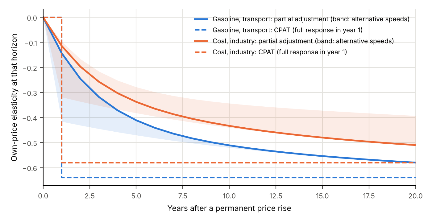
Front-loading overstates early emission cuts and understates early revenue. A tax base that shrinks faster in the model than in the economy yields less modeled revenue in the first years, when budgets are set. For a fuel subsidy reform the error runs the other way on timing: the modeled fall in consumption, and the fiscal gain with it, arrive too early. Phasing a price in gradually, the use for which CPAT’s documentation says the tool is best suited, reduces the error but does not remove it.
CPAT also has almost no switching between fuels outside power. A carbon tax that makes coal dearer than gas cuts coal and gas each by their own elasticities; nothing moves industry from coal to gas or electricity. CPAT’s own panel study recommended adding substitution for specific fuels in specific sectors (working paper, structure).
Comparisons hold up better than levels
Errors that affect every policy and country alike largely cancel when policies are compared. The Total Effective Carbon Price measures a policy mix as the uniform carbon tax that would cut emissions by as much (Brief 6.1). It is a ratio of two cuts computed with the same elasticities, so a common error cancels. In the stylized economy of paper 6.1, replacing the central demand elasticities with CPAT’s raises the cut from a $30 tax by about a third, from 13.4 to 17.5 percent, but moves the Total Effective Carbon Price of a policy mix by only about a tenth, from $36.9 to $33.1 per tonne (working paper, emission cuts and the Total Effective Carbon Price).
So a CPAT ranking of policies or countries is more reliable than a CPAT forecast of tonnes or revenue. The same holds for the back-casts and model comparisons in Brief 5.3: CPAT is best used for ranges and comparisons, and least reliable for near-term levels.
What to do
Finance ministries and development-bank teams using CPAT results: treat near-term cuts as upper bounds. Report cuts and revenue for the first five years with a note that the model front-loads the response, and show a case with road fuel elasticities halved beside the central result. For decisions that hinge on road transport or household electricity, check the elasticities against national evidence.
CPAT’s maintainers: fix the two outliers and the timing. Bring industrial diesel, services gasoline and services electricity into the range of the evidence for those fuels, for example by using their transport or household values. Add separate adjustment speeds for use and for equipment, and report results by year after the reform by default. Rerun the documentation’s own calibration check, which reports road gasoline at −0.77 where the defaults give −0.64.
Everyone updating a policy model: run a fixed validation protocol at every update. Keep a register of verified estimates for each fuel and sector, apart from the model’s own calibration source; classify each default; test what the differences do to a standard scenario; back-cast against past price shocks such as subsidy reforms; and publish every change with its evidence (working paper, protocol).